A worked partially observed fit

library(brms)
library(bicountbrms)

A partially paired design records the second count on every row and the first count on only some of them. binegbin_partialobs() admits both kinds of row under one likelihood: a paired row contributes the full joint probability of the pair, and a row whose first count was never recorded contributes the marginal of the second count, taken from that same joint model.

Partial observation is not censoring in the sense of the brms cens() addition term, which describes a value known to lie in a set. Here the first count was not observed at all, and the likelihood marginalises over its whole support.

Simulating a design with 40% of first counts unrecorded

The complete pair is generated first, and the first count is then withheld on the unpaired rows. Keeping the withheld values aside makes it possible to score the imputation from the model against them at the end, which is not something a real dataset permits.

set.seed(20260826)

n <- 400L
truth <- list(
  mu        = 6,
  lambdaone = 4,
  lambdatwo = 5,
  shapes    = 3,
  shapexone = 2,
  shapextwo = 4
)

n_shared <- rnbinom(n, size = truth$shapes,    mu = truth$mu)
y1_full  <- n_shared + rnbinom(n, size = truth$shapexone, mu = truth$lambdaone)
y2       <- n_shared + rnbinom(n, size = truth$shapextwo, mu = truth$lambdatwo)

# 60% of rows have both counts; on the rest the first count is withheld.
y1_obs <- rbinom(n, 1L, 0.6)

dat <- data.frame(
  y1     = ifelse(y1_obs == 1L, y1_full, 0L),
  y2     = y2,
  y1_obs = y1_obs
)

withheld <- y1_full[y1_obs == 0L]
c(n = n, paired = sum(y1_obs), unpaired = sum(1L - y1_obs))
#>        n   paired unpaired 
#>      400      243      157

The observation flag is a 0/1 integer column, supplied through vint() alongside the second count: vint(y2, y1_obs) binds vint1 to the second count and vint2 to the flag, in the order they are listed.

On an unpaired row, the response column is not read by the likelihood, so any non-negative integer serves as a placeholder; 0 is used above. Do not write NA there. brms drops rows with a missing response before the family is reached, which would discard the second count on exactly the rows the family exists to use.

Fitting

fit <- brm(
  bf(y1 | vint(y2, y1_obs) ~ 1,
     mu ~ 1,
     lambdaone ~ 1, lambdatwo ~ 1,
     shapes ~ 1, shapexone ~ 1, shapextwo ~ 1),
  family   = binegbin_partialobs(),
  stanvars = binegbin_partialobs_stanvars(),
  data     = dat,
  prior    = c(
    prior(normal(2, 1),   class = "Intercept"),
    prior(normal(2, 1),   class = "Intercept", dpar = "lambdaone"),
    prior(normal(2, 1),   class = "Intercept", dpar = "lambdatwo"),
    prior(normal(0, 1.5), class = "Intercept", dpar = "shapes"),
    prior(normal(0, 1.5), class = "Intercept", dpar = "shapexone"),
    prior(normal(0, 1.5), class = "Intercept", dpar = "shapextwo")
  ),
  chains  = 4, iter = 2000, warmup = 1000,
  seed    = 20260826, refresh = 0,
  control = list(adapt_delta = 0.95),
  backend = backend
)

c(divergences = sum(nuts_params(fit, pars = "divergent__")$Value),
  max_rhat    = max(rhat(fit), na.rm = TRUE))
#> divergences    max_rhat 
#>    0.000000    1.005449

The contribution of an unpaired row

An unpaired row is scored by

$P(y_2 = y) = \sum_{k=0}^{y} \mathrm{NB2}(k \mid \mu, \phi_{\text{s}})\, \mathrm{NB2}(y - k \mid \lambda_2, \phi_{x2}),$

which is the joint model with the first count summed out over its whole support. The row is neither dropped nor given a separate univariate model on the second count, either of which would be a different model from the joint model fitted to the paired rows.

Two consequences follow. An unpaired row informs $\mu$ , $\phi_{\text{s}}$ , $\lambda_2$ , $\phi_{x2}$ and any group-level effects. It does not inform $\lambda_1$ or $\phi_{x1}$ , which appear only in the paired branch.

Which parameters an unpaired row informs is a property of the likelihood rather than of this fit. What that property implies for a particular design is taken up further down.

draws <- as.data.frame(fit)

pars <- c(mu        = "b_Intercept",
          lambdaone = "b_lambdaone_Intercept",
          lambdatwo = "b_lambdatwo_Intercept",
          shapes    = "b_shapes_Intercept",
          shapexone = "b_shapexone_Intercept",
          shapextwo = "b_shapextwo_Intercept")

recovery <- do.call(rbind, lapply(names(pars), function(p) {
  x <- exp(draws[[pars[[p]]]])
  data.frame(
    dpar     = p,
    informed = if (p %in% c("lambdaone", "shapexone")) "paired rows" else "every row",
    truth    = truth[[p]],
    median   = median(x),
    lower    = unname(quantile(x, 0.025)),
    upper    = unname(quantile(x, 0.975))
  )
}))

knitr::kable(recovery, digits = 2, row.names = FALSE)

dpar	informed	truth	median	lower	upper
mu	every row	6	4.96	3.61	6.18
lambdaone	paired rows	4	5.08	3.90	6.45
lambdatwo	every row	5	6.15	4.90	7.55
shapes	every row	3	2.46	1.14	4.64
shapexone	paired rows	2	4.41	2.03	10.07
shapextwo	every row	4	5.93	2.98	12.18

Five of the six intervals contain their true value. The interval for $\phi_{x1}$ runs from 2.03 to 10.07 against a true value of 2, missing it at the lower end by 0.03.

The seed was not changed to make the miss disappear. A 95% interval from a correctly specified model excludes the truth 5% of the time by construction, and across six parameters the chance that at least one interval misses is about 26%. One near miss in six is therefore the expected behaviour of a working implementation, not evidence against it. The calibration evidence in this article is the coverage check further down, which is taken over 157 withheld counts rather than over one fit.

The three dispersions have much the wider intervals, because each is estimated from an aggregate mean–variance mismatch rather than from any directly observed quantity.

Imputing the withheld count

posterior_predict() returns a draw of the first count for every row, conditional on the second count recorded there. The observation flag selects a branch of the likelihood; it does not change the prediction. Rows on which the first count was never recorded are therefore predicted in exactly the same way as paired rows. On an unpaired row, the predicted first count is the imputed value of the unrecorded first count.

pp  <- posterior_predict(fit)
idx <- which(dat$y1_obs == 0L)

imp <- data.frame(
  withheld = withheld,
  median   = apply(pp[, idx, drop = FALSE], 2, median),
  lower    = apply(pp[, idx, drop = FALSE], 2, quantile, 0.05),
  upper    = apply(pp[, idx, drop = FALSE], 2, quantile, 0.95)
)
imp$covered <- imp$withheld >= imp$lower & imp$withheld <= imp$upper

c(n_unpaired      = nrow(imp),
  empirical_cover  = mean(imp$covered),
  nominal          = 0.90)
#>      n_unpaired empirical_cover         nominal 
#>     157.0000000       0.8980892       0.9000000

The empirical coverage of the nominal 90% interval is a check on the imputation, not a test of the method: simulating from the model and refitting it makes the coverage nominal by construction when the implementation is correct. It is reported because a departure would indicate an implementation error, and because the interval widths themselves are the quantity a user planning such a design wants to see.

op <- par(mar = c(4.1, 4.1, 2.6, 1.1), bty = "n")
ord <- order(imp$withheld)
plot(imp$withheld[ord], imp$median[ord],
     xlim = range(c(imp$withheld, imp$lower, imp$upper)),
     ylim = range(c(imp$withheld, imp$lower, imp$upper)),
     pch = 16, cex = 0.7, col = "#2D6A7F",
     xlab = "withheld first count", ylab = "predicted first count",
     main = "Imputation against the values withheld from the model")
segments(imp$withheld[ord], imp$lower[ord], imp$withheld[ord], imp$upper[ord],
         col = "#2D6A7F44")
abline(0, 1, lwd = 2, col = "#C4622D")
mtext("segments = 90% predictive interval; line = one to one",
      side = 3, line = -1.1, cex = 0.75, adj = 0.97)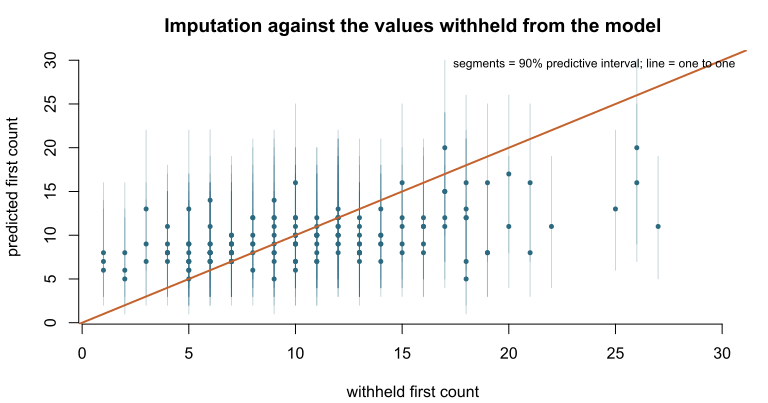

Withheld first counts on the horizontal axis against their predicted values on the vertical, with 90% predictive intervals as vertical segments and a one-to-one line. The points follow a flatter trend than the line, lying above it at low counts and below it at high counts. Most intervals cross the line.

plot of chunk imputation-check

par(op)

The prediction is conditional on the second count, not on the withheld first count. The two counts have only the shared component in common, so the second count constrains the first only through that component and the prediction is shrunk towards the marginal mean of the first count, $\mu + \lambda_1$ , here 10. High withheld counts are therefore under-predicted and low ones over-predicted: the posterior median regressed on the withheld count has slope 0.27 rather than 1. The vertical spread measures what the second count leaves undetermined about the first.

Choosing the fraction of paired rows

$\lambda_1$ and $\phi_{x1}$ appear only in the likelihood term for a paired row, so their precision is set by the number of paired rows rather than by $n$ . The same is true of the between-source bias and the congruence, because both depend on $\lambda_1$ . Where either is the quantity of interest, the number of paired rows should therefore be chosen when the study is designed.

Tying the dispersions of the exclusive and shared components

With few paired rows, a small $\lambda_1$ , or both, shapexone is weakly identified and therefore its posterior stays close to its prior. Where there is no evidence that the two sources differ in the overdispersion of their source-exclusive counts, constraining $\phi_{x1} = \phi_{x2}$ estimates one dispersion for both exclusive components from every row, because $\phi_{x2}$ appears in the likelihood term for both kinds of row. Where the shared component is not expected to differ either, all three dispersions can be constrained to be equal.

Each constraint is imposed by routing the tied dispersions through one non-linear parameter:

# phi_x1 = phi_x2
bf(y1 | vint(y2, y1_obs) ~ 1,
   mu ~ 1,
   lambdaone ~ 1, lambdatwo ~ 1,
   nlf(shapexone ~ shapexx), nlf(shapextwo ~ shapexx),
   shapes ~ 1, shapexx ~ 1, nl = TRUE)

prior(normal(0, 1.5), class = "b", nlpar = "shapexx")

# phi_s = phi_x1 = phi_x2
bf(y1 | vint(y2, y1_obs) ~ 1,
   mu ~ 1,
   lambdaone ~ 1, lambdatwo ~ 1,
   nlf(shapes ~ shapeall), nlf(shapexone ~ shapeall),
   nlf(shapextwo ~ shapeall),
   shapeall ~ 1, nl = TRUE)

prior(normal(0, 1.5), class = "b", nlpar = "shapeall")

The prior on the tied parameter takes class = "b" and nlpar, not class = "Intercept" and dpar; get_prior() on the formula lists the slots. The families and their parameters shows the generated Stan for the two-way tie. Either constraint is an assumption rather than an estimate. Tying trades bias for variance. In the untied model, shapexone is informed by the paired rows alone. In the tied model, the unpaired rows also inform the tied parameter through the second margin, so the posterior variance of the tied parameter is generally smaller. If the tied dispersions differ in truth, the tied parameter is a biased estimate of each tied dispersion. With few paired rows, the 95% interval for $\log\phi_{x1} - \log\phi_{x2}$ under the untied model may contain zero even where $\phi_{x1}$ and $\phi_{x2}$ differ, so the data may not show whether the constraint holds.

Identifying the constructor of a stored fit

fit$family$name is "binegbin" under both constructors. standata(fit) contains vint2 only for a fit from binegbin_partialobs(). For such a fit, fit$family$vars is vint1[n], vint2[n]; for a fit from binegbin(), fit$family$vars is vint1[n], 1. The chunk below prints "vint2" %in% names(standata(fit)) and fit$family$vars for the fit above:

c(has_vint2 = "vint2" %in% names(standata(fit)),
  vars      = paste(fit$family$vars, collapse = ", "))
#>            has_vint2                 vars 
#>               "TRUE" "vint1[n], vint2[n]"