Mapping native parameters to interpretable coordinates

Every joint family in this package — bipois() and binegbin(), each with a _partialobs() constructor for data whose first count is sometimes missing — is built by trivariate reduction. Three independent counts are drawn, and one of the three enters both observed counts:

$y_1 = N_s + N_1 \qquad y_2 = N_s + N_2$

The shared term induces the correlation between the pair. It is never observed, and is marginalised out analytically in the likelihood. $N_1$ and $N_2$ are the source-exclusive counts, each recorded by one source only. The construction and its sources are set out in The families and their parameters.

The widget below shows the same model in both parameterisations, over an expected decomposition and ten simulated pairs.

Two coordinate systems

The dpars a family actually takes are three rates: mu for the shared component, lambdaone and lambdatwo for the two exclusive components. The likelihood is written in terms of these three rates. Increasing the size of the counts moves all three together, so no single rate answers “what is the midpoint of the two expected counts”, “what proportion of the midpoint did both sources record”, or “which source recorded more of the unshared events”.

Those three questions have their own coordinates:

$M$	midpoint of the two expected counts	$\mu + (\lambda_1 + \lambda_2)/2$
$f$	congruence, the mean of the shared component as a proportion of $M$	$\mu / M$
$\beta$	source bias, bounded on $[-1,1]$	$(\lambda_1 - \lambda_2)/(\lambda_1 + \lambda_2)$

Since $\mathrm{E}[y_1] = \mu + \lambda_1$ and $\mathrm{E}[y_2] = \mu + \lambda_2$ , the midpoint is $M = (\mathrm{E}[y_1] + \mathrm{E}[y_2])/2$ , the expected value of the average $(y_1 + y_2)/2$ against which Altman and Bland (1983) plot the difference between two methods of measurement.

The map between them is a bijection, so neither set is more “real”: they are two descriptions of one object. Drag anything below and watch the other five respond.

seed

Interpretable coordinates

Native dpars (what `binegbin()` takes)

Things to try

Turn f up towards 1. Both exclusive rates fall to zero and the two bars converge: the sources agree completely. Now notice what happens to $\beta$ : it stops meaning anything. There are no exclusive events left to be biased, so the bias is unidentified, and the widget flags it and holds the last value rather than snapping to zero. Zero would be a claim (the sources are unbiased) that the state cannot support.

Drag lambdaone alone. $M$ , $f$ and $\beta$ all move, because changing one exclusive rate changes the midpoint, the congruence, and the imbalance simultaneously. This is exactly why the native coordinates are awkward to reason in, and it is much easier to see than to describe.

Turn $\beta$ up and watch $M$ . The two bars separate, but the $M$ rule does not move: it stays at their average, touching neither. The average of the two exclusive rates is $M(1-f)$ for any $\beta$ , so $M$ is pinned to the midpoint whatever the bias. $M$ is a midpoint of what the sources report, not a property of the underlying process.

Compare $\kappa_A$ against $\kappa_X$ . They are near-orthogonal channels. $\kappa_A$ moves the pair up and down together, and cannot alter the difference, because the shared component cancels out of that difference. $\kappa_X$ pulls the pair apart, and drives the whole difference.

Push $\kappa_A$ to 0. The counts do not stop moving. That is the Poisson floor, not determinism: there is no parameter setting that stills the stacks.

Calling the map directly

The arithmetic in the widget is not a separate model: it is the map exported by the package, which you can call directly. The R code below is the authoritative version, and the JavaScript above is checked against it:

library(bicountbrms)

# The widget defaults
binegbin_mfd_to_dpars(
  M      = 12,
  f      = 0.67,
  delta  = atanh(0),
  kappas = 0.6,
  kappax = 1.0
  )
#> $mu
#> [1] 8.04
#> 
#> $lambdaone
#> [1] 3.96
#> 
#> $lambdatwo
#> [1] 3.96
#> 
#> $shapes
#> [1] 2.777778
#> 
#> $shapexone
#> [1] 1
#> 
#> $shapextwo
#> [1] 1

delta is the unbounded log-ratio bias; the $\beta$ in the widget is the bounded $\tanh\delta$ . Going back the other way:

d <- binegbin_mfd_to_dpars(
  M     = 12,
  f     = 0.67,
  delta = 0.3
  )
binegbin_dpars_to_mfd(
  d$mu,
  d$lambdaone,
  d$lambdatwo
  )[c("M", "f", "delta", "beta")]
#> $M
#> [1] 12
#> 
#> $f
#> [1] 0.67
#> 
#> $delta
#> [1] 0.3
#> 
#> $beta
#> [1] 0.2913126

And the degenerate case the widget flags:

# Perfect congruence: no exclusive events, so no bias to identify
binegbin_dpars_to_mfd(
  mu        = 12,
  lambdaone = 0,
  lambdatwo = 0
  )$delta
#> [1] NA

Fitting in these coordinates

Nothing above fits a model: the map and its inverse are coordinate transforms. To fit in $(M, f, \delta)$ you do not need a different family: the reparameterisation is reachable through a non-linear formula with the non-linear parameters logM $= \log M$ , logitf $= \operatorname{logit} f$ and delta $= \delta = \operatorname{artanh} \beta$ .

Every dpar is log-linked, so each formula below is written on the log scale and the link supplies the exp(). That includes the inverse dispersions: writing shapes as $-2\log\kappa_s$ gives $\text{shapes} = e^{-2\log\kappa_s} = 1/\kappa_s^2$ , so the model is estimated in $\kappa$ , the overdispersion the widget above uses, rather than in $\phi$ .

$\kappa = 0$ is the Poisson limit, so a prior on $\kappa$ can shrink towards Poisson. The same reparameterisation was used by Smith et al. (2020).

Priors that default to the simpler model

This section covers priors in the $(M, f, \delta)$ coordinates alone. For the native distributional parameters — which prior goes in which of the class, dpar and nlpar slots, and why brms supplies none of them by default — see Choosing priors, which is the page to read first.

Three of these coordinates have a null at a finite, interpretable zero. The priors below follow from three statements about that null. Zero is the base model: $\kappa = 0$ is a Poisson component, $\delta = 0$ is no bias between the two sources. The effect of a coordinate on the fit grows as the coordinate moves away from zero. The prior density should therefore decrease monotonically away from zero, leaving the data rather than the prior to move the estimate off the base model.

The third statement is Occam’s razor in the sense of Simpson et al. (2017) (their Principle 1), with the scale chosen by what the analyst is willing to permit (their Principle 4). These priors follow the same principles as penalised-complexity priors: a base model at zero, and a density decaying away from it. They are not PC priors in the strict sense, which would require a distance measure derived for this family and a constant-rate assumption on that distance. Neither is established here.

coordinate	base model	prior
$\delta$ (`delta`)	$0$ — no source bias, $\lambda_1 = \lambda_2$	`normal(0, 0.5)`
$\kappa_s$ (`kappas`)	$0$ — Poisson shared component	`normal(0, 1)`, $\kappa \ge 0$
$\kappa_x$ (`kappax`)	$0$ — Poisson exclusive components	`normal(0, 1)`, $\kappa \ge 0$
$\operatorname{logit} f$ (`logitf`)	none — deliberately, see below	`normal(0, 1.5)`

Note what changes on the $\kappa$ scale. In $\phi$ the Poisson limit is $\phi \to \infty$ , so there is no finite point to shrink towards, and a density decaying from zero would pull towards maximum overdispersion. In $\kappa$ the limit is $\kappa = 0$ , so the same density shrinks towards Poisson.

Those four priors transfer between datasets unchanged, because every one of them is scale-free: a log-ratio, two coefficient-of-variation-like quantities, and a proportion. None of them refers to how big the counts are.

The scale sets what the prior permits. On $\kappa$ , lb = 0 makes normal(0, 1) a half-normal, which places 5% of its mass beyond $\kappa = 1.96$ . Since $\kappa$ is the overdispersion standard deviation as a multiple of the mean, that permits a component whose excess variation has a standard deviation about twice its own mean. Whether that is generous or restrictive depends on the counts being modelled. The coordinate is scale-free, so 1.96 means the same thing whatever the counts; whether it is a plausible upper reach for yours is the question to settle before adopting the scale used here.

exponential(1) is an alternative of the same shape, with its maximum at zero, decaying monotonically, and a heavier tail. The two agree at the median to within 3% ( $0.693$ against $0.674$ ) and separate further out: the exponential places 5.0% of its mass beyond $\kappa = 3$ , against 0.27% for the half-normal. Either satisfies the three statements above, so the choice is how much overdispersion the prior permits before the data are consulted. Simpson et al. (2017) §3.2 discusses heavy tails and their numerical behaviour.

Congruence is deliberately not shrunk either way. Both ends of $f$ are degenerate — at $f = 1$ there are no exclusive events left, so $\delta$ becomes unidentified; at $f = 0$ there is no shared component at all — and neither is a natural null for a method comparison. normal(0, 1.5) on $\operatorname{logit} f$ is close to flat over the interior (implied density within 10% of uniform across $f \in [0.1, 0.9]$ ) while falling away at both boundaries, so it declines to take a side. McElreath (2020) makes the same case for that prior on a logit-scale parameter, against the wider normals, which place nearly all their mass near $f = 0$ and $f = 1$ . Fig. S2-1 of Smith et al. (2020) plots the implied densities on the probability scale for normal priors between $\mathrm{N}(0, 1)$ and $\mathrm{N}(0, 3)$ , normal(0, 1.5) among them.

Setting the prior on $M$ from your own counts

$M$ is the only coordinate on the scale of the counts. The others are scale-free, so one recommendation serves any dataset; $M$ takes a prior chosen from the counts being modelled.

normal(4, 1.5) is used below, which covers roughly 3 to 1000 counts per sampling unit and suits the simulated data. For sparser data, lower the mean: normal(0, 2) covers about 0.04 to 27 at 90%.

Move the mean to match your scale rather than raising the SD. logM is $\log M$ , so a normal prior on it is a lognormal on $M$ , and widening that prior pushes mass out to implausible values instead of making it neutral (Smith et al. 2020, Supplement 3, Fig. S3-1).

A prior written on one scale induces a different density on any other. A prior that is weakly informative on one scale need not be weakly informative on another. These priors are written on the linear-predictor scale ( $\log M$ , $\operatorname{logit} f$ ). Check the quantiles of the density each prior induces on the natural scale of $M$ , $f$ and $\beta$ , where those parameters are interpreted (McElreath 2020). Those induced densities are plotted below, with $\delta$ shown as the bounded bias $\beta = \tanh\delta$ , the fractional imbalance between the two exclusive rates:

op <- par(mfrow = c(2, 2), mar = c(4.1, 4.1, 2.6, 1.1), bty = "n")

# logM ~ normal(4, 1.5) on log M  =>  M is lognormal
M <- seq(0.5, 250, length.out = 200)
plot(M, dlnorm(M, 4, 1.5), type = "l", lwd = 2, col = "#2D6A7F",
     xlab = "M  (midpoint)", ylab = "density",
     main = "log M ~ normal(4, 1.5)")

# logitf ~ normal(0, 1.5) on logit f  =>  Jacobian 1 / (f (1 - f))
f <- seq(0.001, 0.999, length.out = 200)
plot(f, dnorm(qlogis(f), 0, 1.5) / (f * (1 - f)), type = "l", lwd = 2,
     col = "#8A8072", ylim = c(0, 1.4),
     xlab = "f  (congruence)", ylab = "density",
     main = "logit f ~ normal(0, 1.5)")
abline(h = 1, lty = 3)                      # uniform, for comparison
mtext("dotted line = uniform", side = 3, line = -1.1, cex = 0.7, adj = 0.97)

# delta ~ normal(0, 0.5); beta = tanh(delta)
beta <- seq(-0.985, 0.985, length.out = 200)
plot(beta, dnorm(atanh(beta), 0, 0.5) / (1 - beta^2), type = "l", lwd = 2,
     col = "#C4622D",
     xlab = expression(beta == tanh(delta) ~ "  (source bias)"),
     ylab = "density", main = "shrinks to no bias")
abline(v = 0, lty = 3)

# kappas, kappax ~ normal(0, 1) with lb = 0, i.e. half-normal;
# kappa = 0 IS the Poisson limit
k <- seq(0, 4, length.out = 200)
plot(k, 2 * dnorm(k, 0, 1), type = "l", lwd = 2, col = "#6B5D4F",
     xlab = expression(kappa ~ "  (overdispersion)"),
     ylab = "density", main = "shrinks to Poisson")
abline(v = 0, lty = 3)
mtext(expression(kappa == 0 ~ "is Poisson"), side = 3, line = -1.1,
      cex = 0.7, adj = 0.97)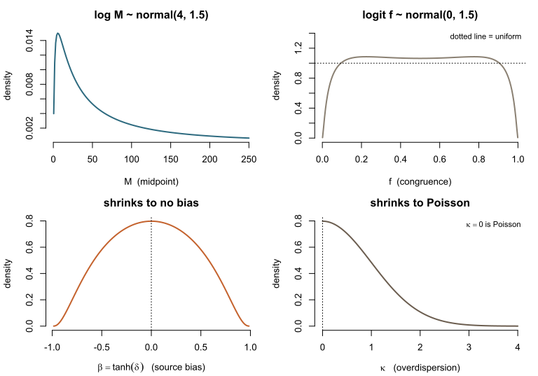

Four panels showing the implied prior density on the interpretable scale: midpoint M, congruence f, bounded bias beta, and overdispersion kappa.

plot of chunk prior-pushforward


par(op)

The priors on $\beta$ and $\kappa$ concentrate mass at the null and decay away from it. The prior on $f$ is flat across the interior and declines only where the model degenerates. None is tight enough to dominate 400 observations, and the fit below tests that claim.

Simulate a pair of counts from known coordinates:

library(brms)
library(bicountbrms)

set.seed(20260731)

M_true  <- 12
f_true  <- 0.67
d_true  <- 0.3
ks_true <- 0.5
kx_true <- 0.6

truth <- binegbin_mfd_to_dpars(
  M      = M_true,
  f      = f_true,
  delta  = d_true,
  kappas = ks_true,
  kappax = kx_true
)

n  <- 400
Ns <- rnbinom(n, size = truth$shapes, mu = truth$mu)

dat <- data.frame(
  y1 = Ns + rnbinom(n, size = truth$shapexone, mu = truth$lambdaone),
  y2 = Ns + rnbinom(n, size = truth$shapextwo, mu = truth$lambdatwo)
)

unlist(truth)
#>        mu lambdaone lambdatwo    shapes shapexone shapextwo 
#>  8.040000  5.113598  2.806402  4.000000  2.777778  2.777778

Fit. Every prior either shrinks towards the simpler model or is centred away from the truth, so the posterior is driven by the data rather than the prior:

fit <- brm(
  bf(y1 | vint(y2) ~ 1, nl = TRUE) +
    nlf(mu        ~ logM + log_inv_logit(logitf)) +
    nlf(lambdaone ~ log(2) + logM + log_inv_logit(-logitf) +
                    log_inv_logit( 2 * delta)) +
    nlf(lambdatwo ~ log(2) + logM + log_inv_logit(-logitf) +
                    log_inv_logit(-2 * delta)) +
    nlf(shapes    ~ -2 * log(kappas)) +
    nlf(shapexone ~ -2 * log(kappax)) +
    nlf(shapextwo ~ -2 * log(kappax)) +
    lf(logM ~ 1, logitf ~ 1, delta ~ 1, kappas ~ 1, kappax ~ 1),
  family   = binegbin(),
  stanvars = binegbin_stanvars(),
  data     = dat,
  prior    = c(
    prior(normal(4, 1.5), class = "b", nlpar = "logM"),
    prior(normal(0, 1.5), class = "b", nlpar = "logitf"),
    prior(normal(0, 0.5), class = "b", nlpar = "delta"),
    prior(normal(0, 1),   class = "b", nlpar = "kappas", lb = 0),
    prior(normal(0, 1),   class = "b", nlpar = "kappax", lb = 0)
  ),
  chains  = 2,
  iter    = 2000,
  warmup  = 1000,
  refresh = 0,
  seed    = 20260731
)

The coordinates are read off the posterior directly: logM exponentiates to $M$ , logitf inverse-logits to $f$ , and delta and the two kappas are the coordinates themselves, with no transformation needed:

post <- as_draws_df(fit)

qi <- function(x) c(median(x), quantile(x, c(0.05, 0.95)))

recovered <- rbind(
  M      = qi(exp(post$b_logM_Intercept)),
  f      = qi(plogis(post$b_logitf_Intercept)),
  delta  = qi(post$b_delta_Intercept),
  kappas = qi(post$b_kappas_Intercept),
  kappax = qi(post$b_kappax_Intercept)
)
colnames(recovered) <- c("median", "q5", "q95")

knitr::kable(
  cbind(truth = c(M_true, f_true, d_true, ks_true, kx_true), recovered),
  digits = 3
)

	truth	median	q5	q95
M	12.00	12.185	11.764	12.636
f	0.67	0.662	0.598	0.709
delta	0.30	0.282	0.222	0.346
kappas	0.50	0.509	0.444	0.589
kappax	0.60	0.541	0.417	0.674

Because the map is a bijection, the same posterior can be read in native dpars without refitting: push the draws back through binegbin_mfd_to_dpars():

back <- binegbin_mfd_to_dpars(
  M     = exp(post$b_logM_Intercept),
  f     = plogis(post$b_logitf_Intercept),
  delta = post$b_delta_Intercept
)

knitr::kable(
  data.frame(
    dpar   = c("mu", "lambdaone", "lambdatwo"),
    truth  = c(truth$mu, truth$lambdaone, truth$lambdatwo),
    median = vapply(back, median, numeric(1))
  ),
  digits = 3,
  row.names = FALSE
)

dpar	truth	median
mu	8.040	8.084
lambdaone	5.114	5.258
lambdatwo	2.806	2.978

A random effect on logM estimates how much groups differ in midpoint, and a random effect on logitf estimates how much they differ in congruence. Those are separable in these coordinates and entangled in the native dpars, where a group effect on mu alone changes the midpoint and the congruence at once.

The JavaScript is an independent implementation of the generative model: it draws from the same trivariate reduction, but it is not the likelihood, and no part of the inference performed by the package runs in your browser. It uses the rate map tested in test-mfd.R; the sampler is illustrative. Treat the picture as intuition, and the R above as the specification.

The widget also shows ONE overdispersion dial for the exclusive components. binegbin() estimates two, shapexone and shapextwo, and the (M, f, delta) coordinates this article is about use one kappax for both – so the dial sets both to the same value, which is the symmetric special case. Freeing them means giving each its own nlf() line, as the fit above would if the two margins were allowed to differ.

References

Altman, Douglas G., and J. Martin Bland. 1983. “Measurement in Medicine: The Analysis of Method Comparison Studies.” Journal of the Royal Statistical Society. Series D (The Statistician) 32 (3): 307–17. https://doi.org/10.2307/2987937.

McElreath, Richard. 2020. Statistical Rethinking: A Bayesian Course with Examples in R and Stan. 2nd ed. Chapman; Hall/CRC. https://doi.org/10.1201/9780429029608.

Simpson, Daniel, Håvard Rue, Andrea Riebler, Thiago G. Martins, and Sigrunn H. Sørbye. 2017. “Penalising Model Component Complexity: A Principled, Practical Approach to Constructing Priors.” Statistical Science 32 (1): 1–28. https://doi.org/10.1214/16-STS576.

Smith, A. N. H., D. Acuña-Marrero, P. Salinas-de-León, E. S. Harvey, M. D. M. Pawley, and M. J. Anderson. 2020. “Instantaneous Vs. Non-Instantaneous Diver-Operated Stereo-Video (DOV) Surveys of Highly Mobile Sharks in the Galápagos Marine Reserve.” Marine Ecology Progress Series 649: 111–23. https://doi.org/10.3354/meps13447.