The STAGE Likelihood

Overview

This vignette describes the likelihood and parameterisation used in the STAGE model.

STAGE is a hierarchical Bayesian generative model designed to estimate a transition point $m_{50}$ on variable $x$ between two classes—for example, the length at which individuals transition from immature to mature. The model produces a posterior distribution for $m_{50}$, representing the value of $x$ at which the probabilities $\Pr(y=0)$ and $\Pr(y=1)$ are equal. The model can also be used to derive other useful quantities (such as class probabilities $\Pr(y = 1 \mid x)$).

Conceptually, STAGE is a Bayesian generative classifier for estimating a transition point (e.g. length at maturity). Each class is fit with an asymmetric plateau–Gaussian density:

• the lower class has a uniform plateau followed by a Gaussian tail down into the transition,
• the higher class has a Gaussian tail up out of the transition followed by a uniform plateau.

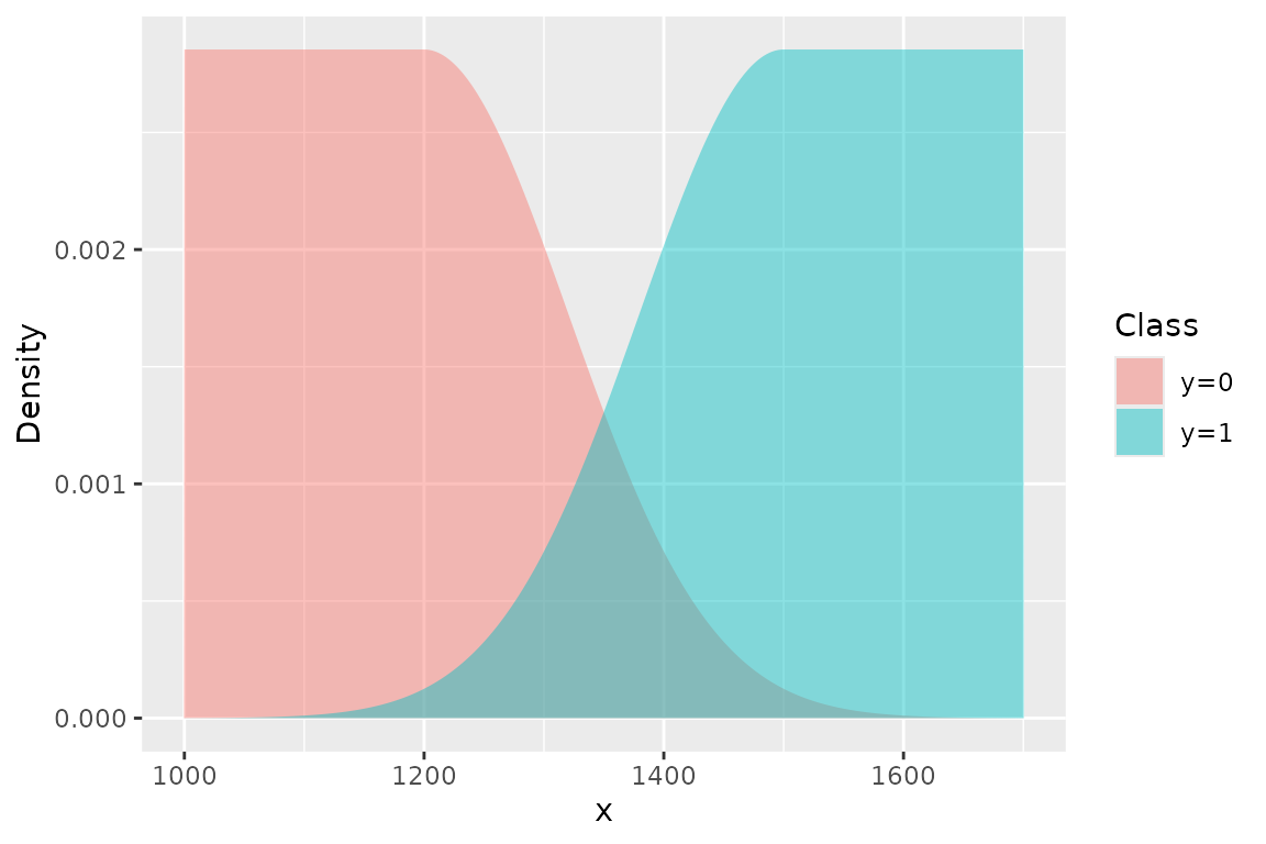
This construction focuses inference on the overlap region and prevents distant observations (e.g. very small immatures, very large matures) from unduly influencing the transition point.

The central idea is to model each class with a piecewise density that combines a uniform plateau in regions far from the transition, and a Gaussian tail in the transition region. The left group ($y = 0$) is modelled with a uniform on the left that begins at the lower truncation value $L$. The distribution remains flat until it approaches the transition range, at which point the distribution declines according to a Gaussian. The right group ($y = 1$) is a mirror image of the left—it increases according to a Gaussian distribution and then levels off to a uniform, terminating at the upper truncation value $U$.

The model focuses inference on the transition zone, where the values of $x$ of the two classes overlap, and down-weights observations that are biologically uninformative because they are far away from the transition point.

The uniform–Gaussian pdf used here is adapted from a plateau proposal distribution combining a uniform and two Gaussians described by Lau & Krumscheid (2022).

Model summary

We observe pairs $(x_i, y_i)$ for $i = 1, \dots, N$, where

• $x_i$ is a continuous covariate (e.g., length), truncated to an interval $[L, U]$, and
• $y_i \in \{0, 1\}$ is a binary indicator of state (e.g., immature / mature).

The model assumes that the distribution of $x$ conditional on state is piecewise:

• For $y = 0$ (immature individuals), the distribution of $x$ is approximately uniform up to a point $\mu_0$, after which it follows a Gaussian decay.
• For $y = 1$ (mature individuals), the distribution is Gaussian below a point $\mu_1$, and uniform above $\mu_1$ up to the upper truncation $U$.

The transition point $m_{50}$ is the value of $x$ where the probability of observing either class is equal:

$$\Pr(y = 0 \mid x = m_{50}) = \Pr(y = 1 \mid x = m_{50}).$$

Additional parameters govern the width and sharpness of the transition:

• $d$ controls the distance between $\mu_0$ and $\mu_1$ (the width of the transition region),
• $\sigma$ (denoted sigma_x in the Stan code) controls the spread (standard deviation) of the Gaussian tails.

By allowing different behaviours on either side of the transition, the model can capture asymmetric transition patterns: the immature class can decline towards the transition at a different rate than the mature class rises out of it.

This is particularly useful in settings where:

• the boundary between classes is not sharp, and
• the data exhibit gradual overlap between the two classes.

Likelihood

The likelihood is built from two unnormalised log-density functions for the two classes. We work on the log scale for numerical stability and then subtract log-normalising constants to obtain valid densities.

Let $\ell_0(x)$ and $\ell_1(x)$ denote the unnormalised log-densities for $y = 0$ and $y = 1$, respectively. The corresponding (unnormalised) densities are $\tilde f_k(x) = \exp\{\ell_k(x)\}$.

We restrict attention to the truncated interval $[L, U]$; the densities are zero outside this range.

Lower class ($y = 0$)

For $y_i = 0$, the unnormalised piecewise log-density is

$$\ell_0(x_i \mid \mu_0, \sigma, L) = \begin{cases} 0 & \text{if } L \leq x_i \leq \mu_0, \\ -\dfrac{(x_i - \mu_0)^2}{2\sigma^2} & \text{if } x_i > \mu_0 . \end{cases}$$

Here:

• the plateau region $[L, \mu_0]$ has constant log-density 0 (density 1),
• the tail region $x_i > \mu_0$ decays according to a Gaussian kernel.

Any constant could be added to $\ell_0(\cdot)$ without changing the posterior; we fix the plateau at 0 so that the plateau density is 1 after exponentiation.

Higher class ($y = 1$)

For $y_i = 1$, the unnormalised log-density is

$$\ell_1(x_i \mid \mu_1, \sigma, U) = \begin{cases} -\dfrac{(x_i - \mu_1)^2}{2\sigma^2} & \text{if } x_i < \mu_1, \\ 0 & \text{if } \mu_1 \leq x_i \leq U . \end{cases}$$

Now:

• the Gaussian tail is below $\mu_1$, and
• the plateau covers the upper region $[\mu_1, U]$.

In both cases we have a plateau–Gaussian shape: a flat density where the class “dominates” and a Gaussian tail in the transition region where the other class is present.

Normalisation constants

To convert $\tilde f_k(x) = \exp\{\ell_k(x)\}$ into proper probability density functions on $[L, U]$, we divide by constants $C_0$ and $C_1$ chosen so that the densities integrate to 1.

For the immature class ($y = 0$):

$$C_0 = \int_L^{\mu_0} 1 \, dx + \int_{\mu_0}^{\infty} \exp\!\left( -\frac{(x - \mu_0)^2}{2\sigma^2} \right) dx = (\mu_0 - L) + \frac{\sqrt{2\pi}\,\sigma}{2}.$$

For the mature class ($y = 1$):

$$C_1 = \int_{-\infty}^{\mu_1} \exp\!\left( -\frac{(x - \mu_1)^2}{2\sigma^2} \right) dx + \int_{\mu_1}^{U} 1 \, dx = \frac{\sqrt{2\pi}\,\sigma}{2} + (U - \mu_1).$$

Intuitively:

• $(\mu_0 - L)$ and $(U - \mu_1)$ are the widths of the uniform plateaus,
• $\sqrt{2\pi}\,\sigma / 2$ is the contribution from the half-Gaussian tail.

The corresponding log-likelihood contribution for observation $i$ is

$$\log \mathcal{L}_i = \begin{cases} \ell_0(x_i) - \log C_0 & \text{if } y_i = 0, \\ \ell_1(x_i) - \log C_1 & \text{if } y_i = 1. \end{cases}$$

Summing over all observations,

$$\log p(x, y \mid m_{50}, d, \sigma) = \sum_{i=1}^{N} \big[ \ell_{y_i}(x_i) - \log C_{y_i} \big],$$

which is exactly the likelihood implemented in the Stan code used by fit_stage().

Prior specification

The priors reflect prior beliefs about plausible transition points and transition widths in typical length-at-maturity problems. In practice, these are defaults that should be adapted to the scale of the data and prior biological knowledge.

By default, STAGE uses weakly informative normal priors:

• Transition point $m_{50}$ (Stan parameter m50):

$$m_{50} \sim \mathcal{N}(1300, 50),$$

which centres the transition point around 1300 (mm) with moderate uncertainty.

• Transition width $d$:

$$d \sim \mathcal{N}(100, 100),$$

which allows the width of the overlap region to vary around 100 units with a wide spread. Note that $d$ is the distance between the class-specific Gaussian centres.

• Gaussian spread $\sigma$ (Stan parameter sigma_x):

$$\sigma \sim \mathcal{N}(100, 50),$$

representing prior beliefs about the scale of variability in the transition tails.

Because $d$ and sigma_x are constrained to be positive in the Stan model, their Normal priors are effectively half-Normal distributions (the prior mass below zero is folded onto the positive half).

In practice, you should adapt these priors to your scale (e.g., lengths, ages) and prior biological knowledge. The STAGE implementation allows you to pass in hyperparameters via helper functions such as stage_priors().

Transformed parameters

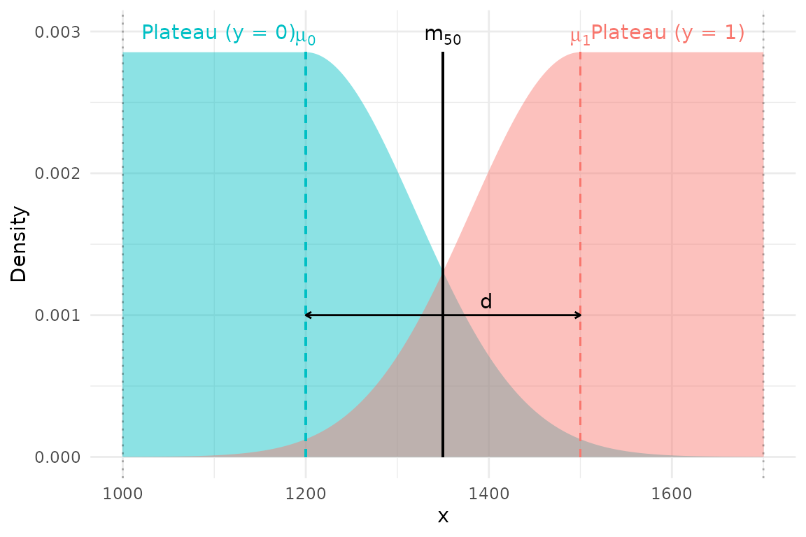
The Gaussian “centres” for the two classes are defined in terms of the transition point $m_{50}$ and the width parameter $d$:

$$\mu_0 = m_{50} - \frac{d}{2}, \qquad \mu_1 = m_{50} + \frac{d}{2}.$$

Thus:

• $d$ controls the distance between the immature and mature Gaussian means,
• $m_{50}$ is the midpoint between them.

From class densities to class probabilities (Bayes rule)

The likelihood above defines the class-conditional densities $f_0(x) = p(x \mid y = 0)$ and $f_1(x) = p(x \mid y = 1)$ on $[L, U]$, obtained by normalising the unnormalised densities $\tilde f_k(x) = \exp\{\ell_k(x)\}$ with the constants $C_k$.

To obtain the probability that an individual with a particular $x$ value is in the higher class ($y = 1$), we use Bayes rule:

$$\Pr(y = 1 \mid x) = \frac{\pi_1 f_1(x)}{\pi_0 f_0(x) + \pi_1 f_1(x)},$$

and similarly

$$\Pr(y = 0 \mid x) = \frac{\pi_0 f_0(x)}{\pi_0 f_0(x) + \pi_1 f_1(x)},$$

where $\pi_0$ and $\pi_1$ are the prior class probabilities (e.g., prior probabilities of being immature or mature before seeing $x$).

In many applications, such as estimating length-at-maturity, we are interested in a transition point that is not driven by sample sizes or prevalence, so it is natural to use equal class priors, $\pi_0 = \pi_1 = 1/2$. In that case, Bayes rule simplifies to

$$\Pr(y = 1 \mid x) = \frac{f_1(x)}{f_0(x) + f_1(x)}, \qquad \Pr(y = 0 \mid x) = \frac{f_0(x)}{f_0(x) + f_1(x)}.$$

These are the class probabilities that the STAGE model uses for prediction, and they are what you see when you plot $\Pr(y = 1 \mid x)$ as a function of $x$.

Connection to $m_{50}$

By definition, the transition point $m_{50}$ is the value of $x$ where the two classes are equally probable:

$$\Pr(y = 0 \mid x = m_{50}) = \Pr(y = 1 \mid x = m_{50}) = \frac{1}{2}.$$

Using Bayes rule with equal class priors, this equality is equivalent to

$$f_0(m_{50}) = f_1(m_{50}),$$

i.e. the two normalised class densities are equal at $m_{50}$.

Why $m_{50}$ is the midpoint between $\mu_0$ and $\mu_1$. In the transition region ($\mu_0 < x < \mu_1$), both unnormalised densities take Gaussian form:

$$\tilde f_0(x) = \exp\!\left(-\frac{(x - \mu_0)^2}{2\sigma^2}\right), \qquad \tilde f_1(x) = \exp\!\left(-\frac{(x - \mu_1)^2}{2\sigma^2}\right).$$

Since both Gaussians share the same $\sigma$, the unnormalised densities are equal at the arithmetic midpoint $x^* = (\mu_0 + \mu_1)/2 = m_{50}$. With equal class priors, the normalising constants $C_0$ and $C_1$ cancel in the likelihood ratio, so the 50% crossing point is exactly $m_{50}$ regardless of the survey bounds $L$ and $U$. This is the key invariance property: changing the sampling domain does not shift the estimated transition point.

Visualising a single STAGE transition

We can visualise a simple STAGE configuration, showing:

• the immature and mature densities, and
• the resulting transition probability $\Pr(y=1 \mid x)$.

Relationship to the stage implementation

In the stage package:

• The single-population model directly samples m50 ($m_{50}$), d, and sigma_x ($\sigma$). The transition point is a primary sampling parameter, not a derived quantity.
• The multi-population (hierarchical) model introduces population-specific transition points via a random-effects structure: $$\texttt{m50\_pop}[j] = m_{50} + z_j \, \sigma_\alpha,$$ where $m_{50}$ is the global mean transition point, $z_j$ are standard-normal effects, and $\sigma_\alpha$ is the population-level standard deviation.

The Stan code used in fit_stage() is a direct implementation of the likelihood and parameterisation described above.

Future vignettes will provide a more detailed walk-through of the Stan code and extensions such as alternative priors and model comparison.

References

Lau, F. Din-Houn, and Sebastian Krumscheid. 2022. “Plateau Proposal Distributions for Adaptive Component-Wise Multiple-Try Metropolis.” METRON 80 (3): 343–70. https://doi.org/10.1007/s40300-022-00235-y.