Chapter 8:
Analysis of Variance (ANOVA) and Analysis of Covariance (ANCOVA)

Learning Objectives

Define and understand an ANOVA
Use a one-way ANOVA on example data
Understand and calculate an ANOVA table
Describe Tukey’s post hoc tests and assumptions of ANOVAs
Understand the difference between one-way and two-way ANOVAs

ANOVA

Analysis of variance, or ANOVA, is an approach to comparing data with multiple means across different groups, and allows us to see patterns and trends within complex and varied data.
Used for categorical or grouped data.
Often data from experiments (treatments make good factors).
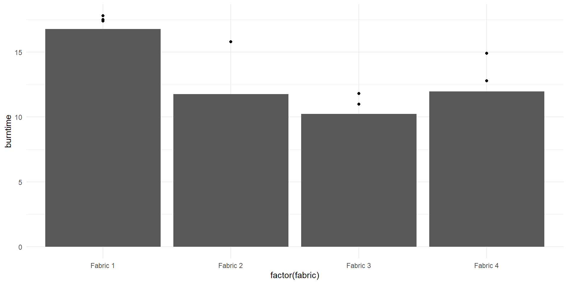
EDA bar, points, or box plots are options to show differences between groups.

One-way (single factor) ANOVA model

fabric burn-time data

fabric 1	fabric 2	fabric 3	fabric 4
17.8	11.2	11.8	14.9
16.2	11.4	11	10.8
17.5	15.8	10	12.8
17.4	10	9.2	10.7
15	10.4	9.2	10.7

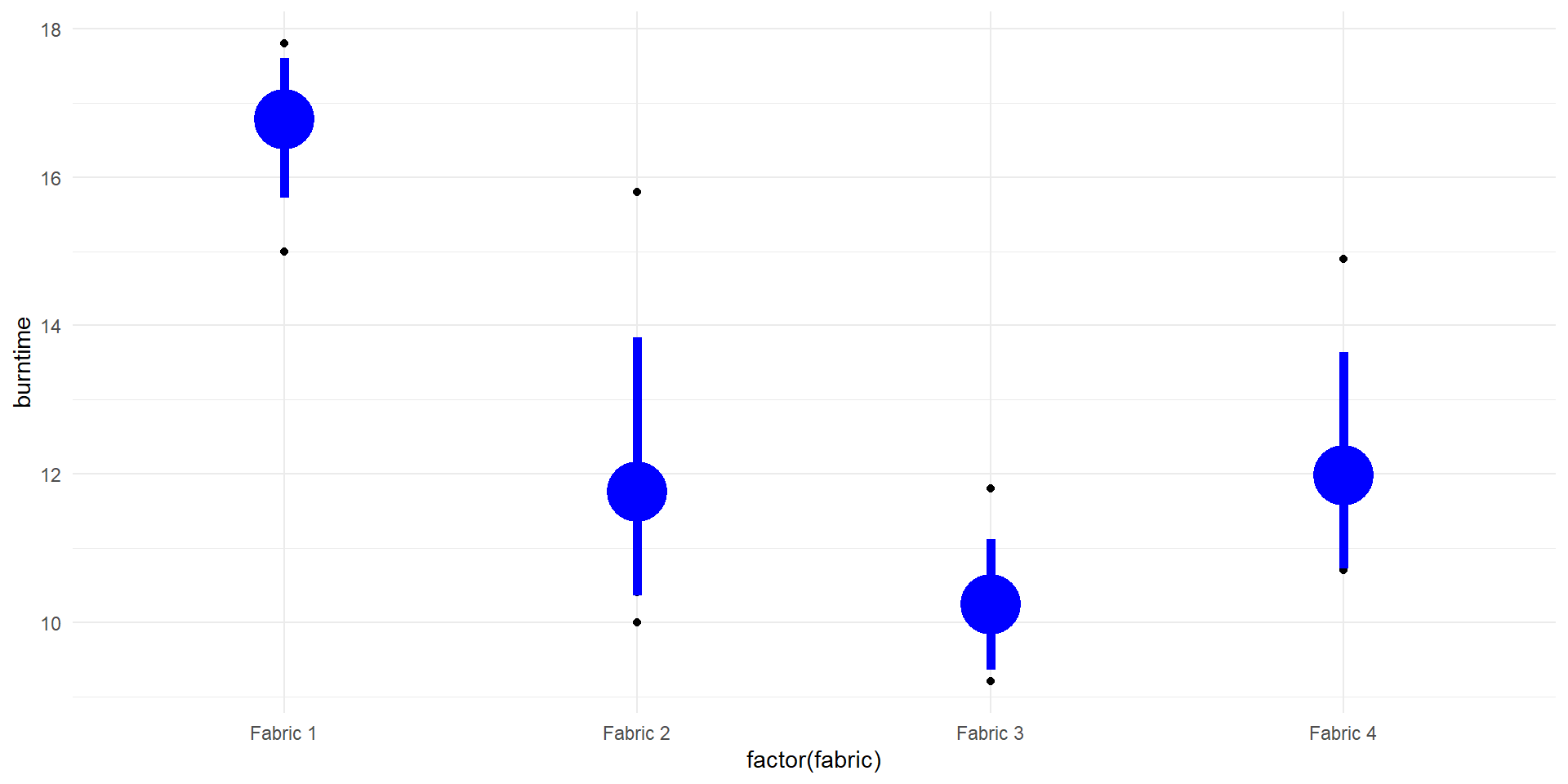
Can we regard the mean burn times of the four fabrics as equal?
- fabric 1 seems to take longer time to burn
Start with hypotheses and EDA to visualize groups

One-way ANOVA Hypotheses

\(H_0\): The mean burn times are equal for the four fabrics
\(H_a\): The mean burn time of at least one fabric is different.

One-way ANOVA

fabric=read.table("../data/fabric.txt", header=TRUE, sep="\t")
fabric |>
  ggplot(aes(x=factor(fabric), y=burntime))+
  geom_point()+
  stat_summary(fun.data = "mean_cl_boot", colour = "blue", linewidth = 2, size = 3)

fabric |>
  ggplot(aes(x=factor(fabric), y=burntime))+
  geom_point()+
  stat_summary_bin(fun = "mean", geom = "bar", orientation = 'x')

One-way (single factor) ANOVA model

ANOVA table

observation = mean + effect + error

SS Total = SS Factor + SS Error

summary(aov(burntime ~ fabric, data = fabric))

            Df Sum Sq Mean Sq F value   Pr(>F)    
fabric       3 120.50   40.17   13.89 0.000102 ***
Residuals   16  46.26    2.89                     
---
Signif. codes:  0 '***' 0.001 '**' 0.01 '*' 0.05 '.' 0.1 ' ' 1

fabric effect on burntime is highly significant.
- In other words, the null hypothesis of equal mean burntime is rejected.
  - Or alternatively the mean burntime is different for at least one fabric

ANOVA table

How are these values calculated?

            Df Sum Sq Mean Sq F value   Pr(>F)    
fabric       3 120.50   40.17   13.89 0.000102 ***
Residuals   16  46.26    2.89                     
---
Signif. codes:  0 '***' 0.001 '**' 0.01 '*' 0.05 '.' 0.1 ' ' 1

SS	df	MeanSq
FACTOR	k-1	FACTOR SS/(k-1)
ERROR	n-k	ERROR SS/(n-k)
TOTAL	n-1	TOTAL SS/(n-1)

ANOVA table

Calculating F values of a factor:

\(F = \frac{MS_{Factor}}{MS_{Error}}\)

SS	df	MeanSq
FACTOR	k-1	FACTOR SS/(k-1)
ERROR	n-k	ERROR SS/(n-k)
TOTAL	n-1	TOTAL SS/(n-1)

ANOVA table practice

SS	df	MeanSq	F- value
FACTOR	k-1	FACTOR SS/(k-1)	MSF/MSE
ERROR	n-k	ERROR SS/(n-k)
TOTAL	n-1	TOTAL SS/(n-1)

	SS	df	MeanSq	F- value	P-value
fabric	120.5
Residuals	46.3
TOTAL

Reminder on P values

In null-hypothesis significance testing, the p-value is the probability of obtaining test results at least as extreme as the result actually observed, under the assumption that the null hypothesis is correct.

A very small p-value means that such an extreme observed outcome would be very unlikely under the null hypothesis.

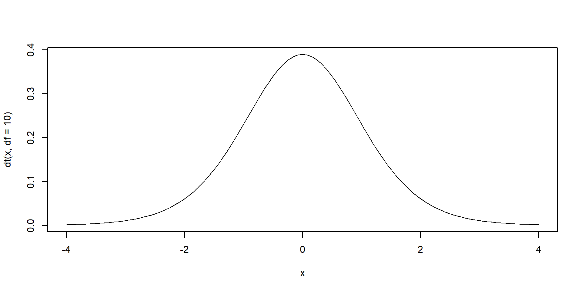
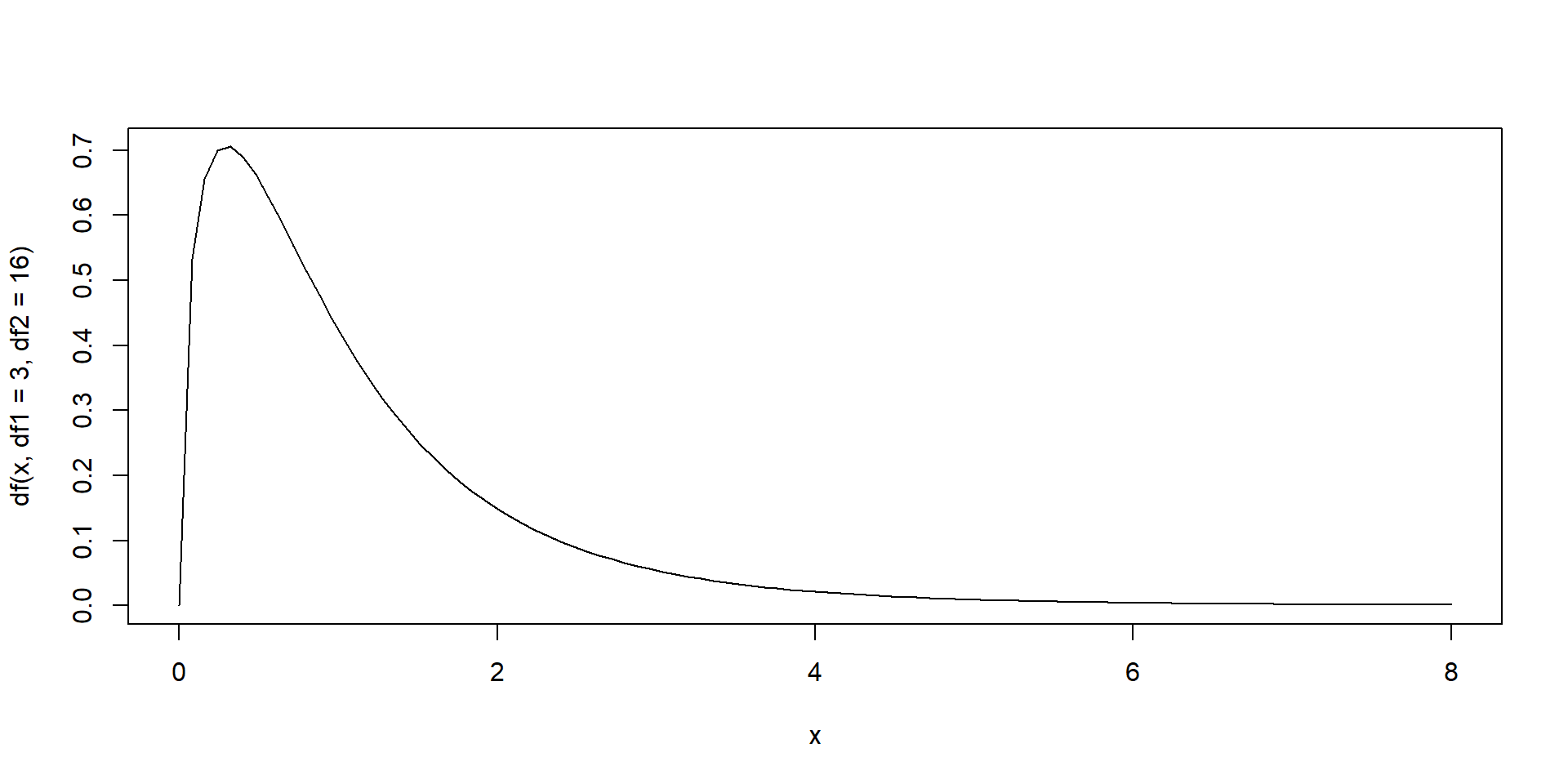
We calculate them based on our theoretical sampling distributions (normal, \(t\), \(F\), \(\chi^2\))

Reminder of Sampling Distributions

A sampling distribution is a probabilistic model of sampling variation–it describes the behaviour of some sample statistic

For a normal population, when the population parameters and are known, we can easily derive the sampling distributions of the sample mean or sample variance.

When the population parameters are unknown, we have to estimate them from data.

Reminder of Sampling Distributions

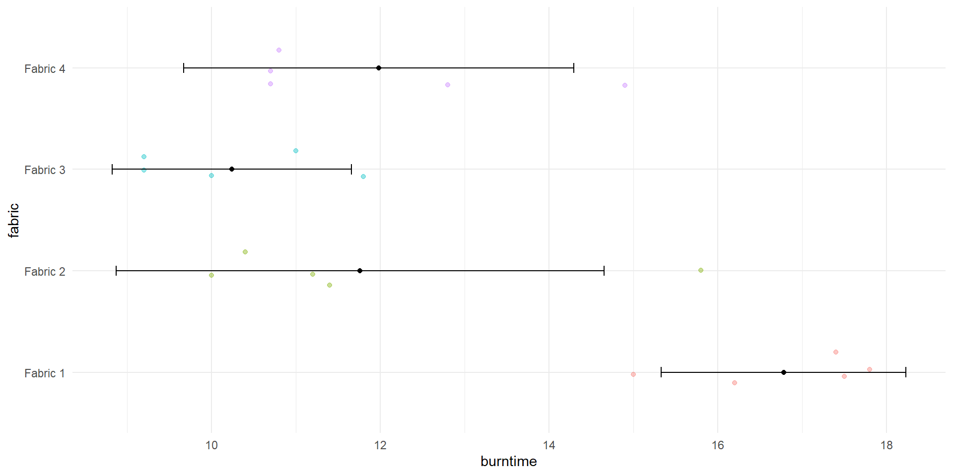
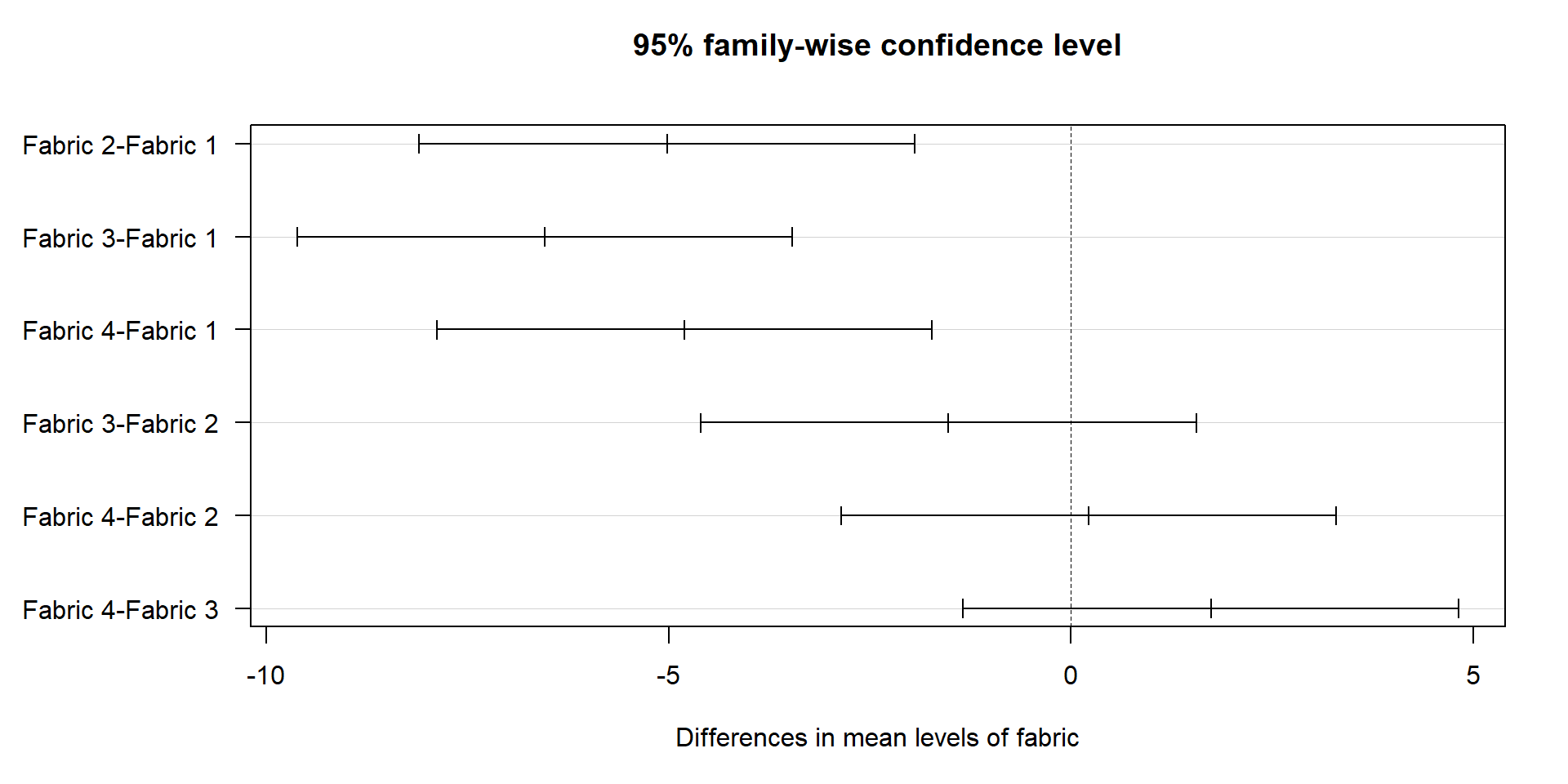
Graphical comparison of means

The graph below shows individual 95% confidence intervals for the fabric means

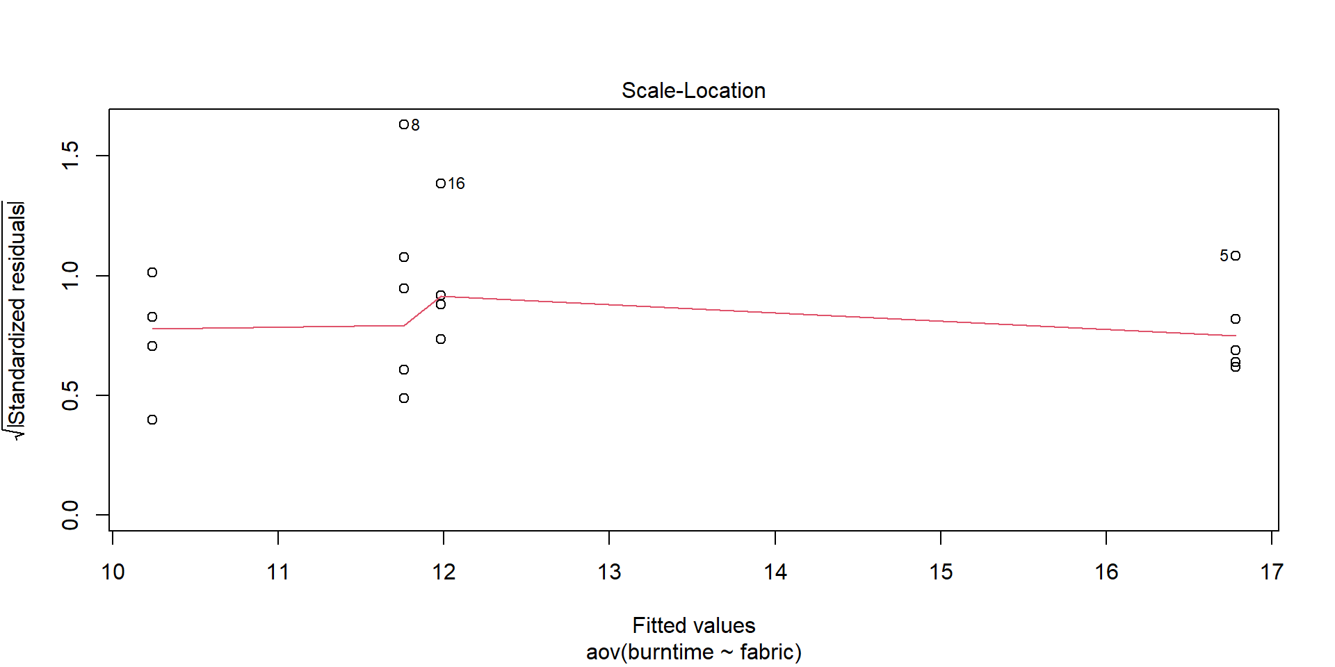
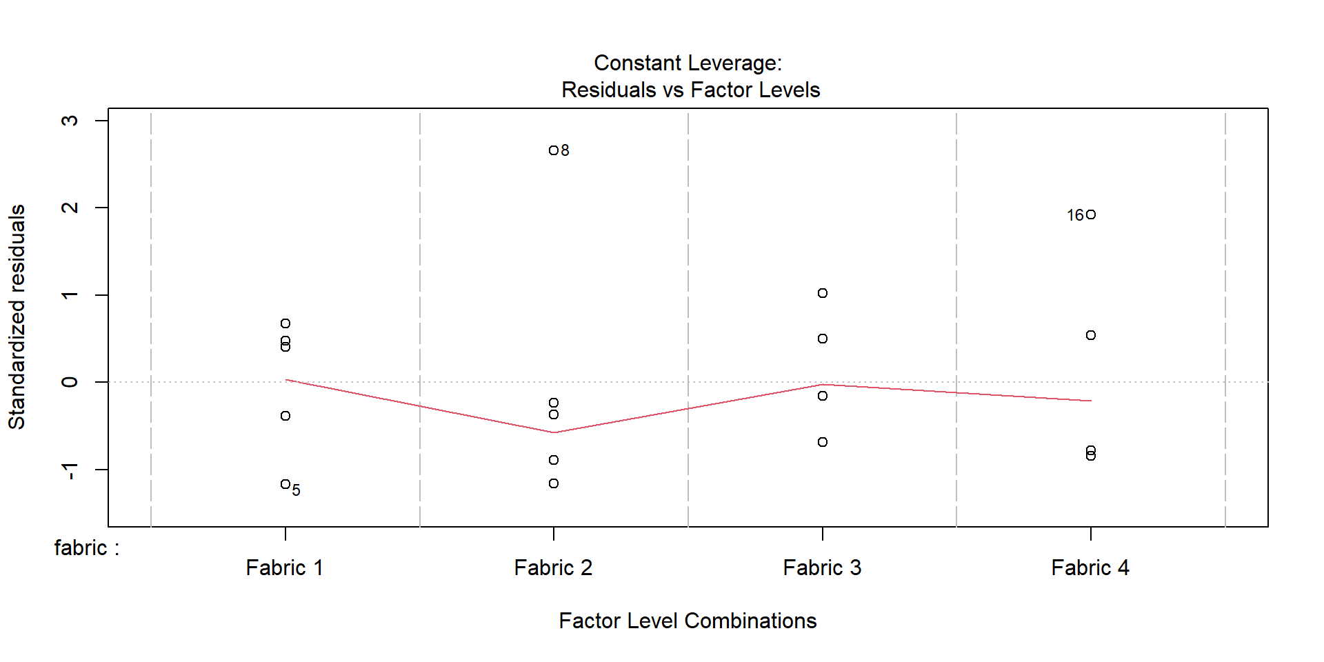
One-way ANOVA model Assumptions

Residuals are randomly and normally distributed
Residuals must be independent of means.
- If SD increases with mean, try square root or logarithmic transformation.
The ANOVA model assumes equal SD for the treatments.
If experimental errors are more in some subgroups, divide the problem into separate ones.
Positive correlation among residuals leads to under estimation of error variance; negative correlation leads to overestimation.

These assumptions are harder to validate to small experimental design data

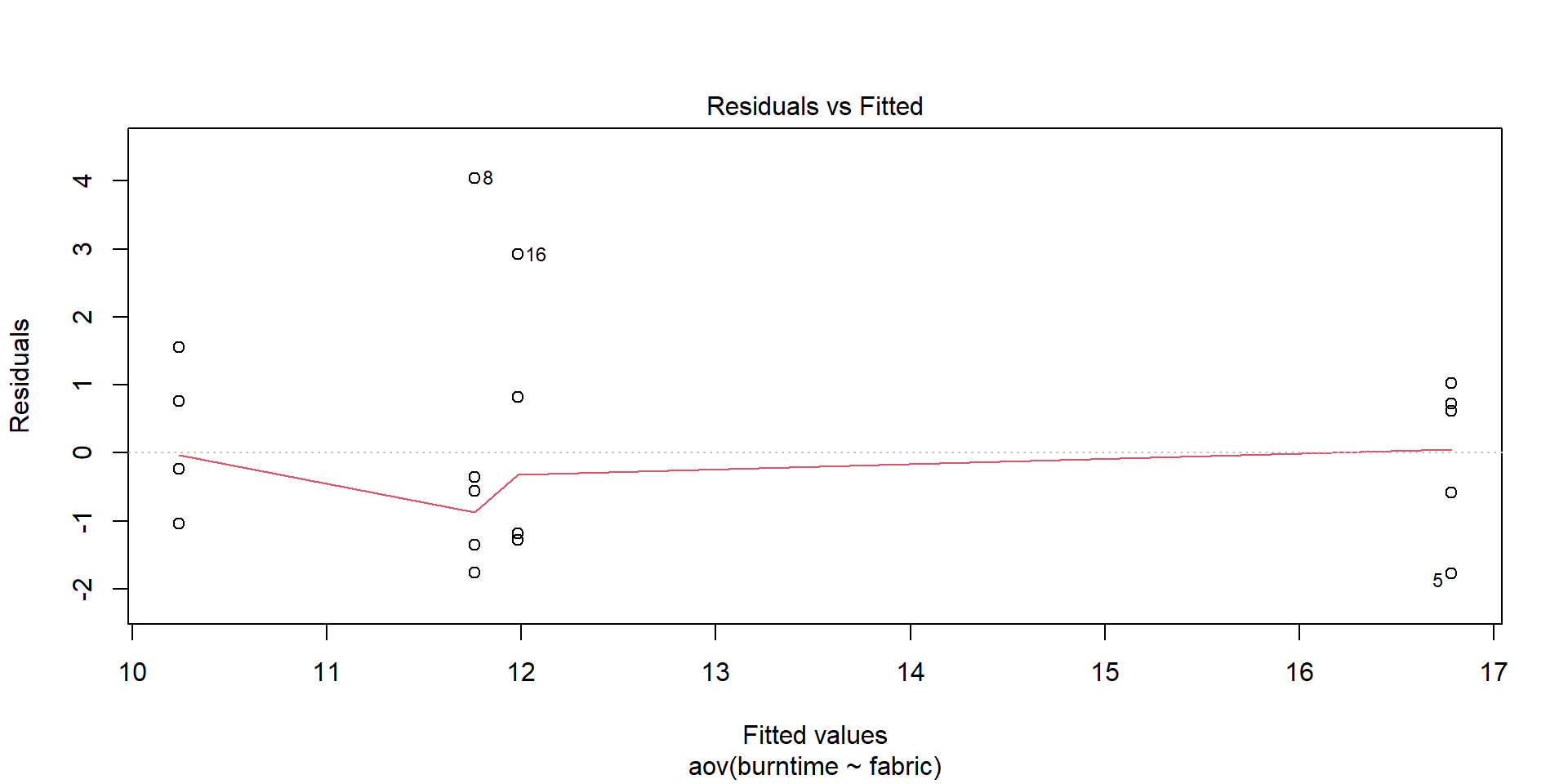
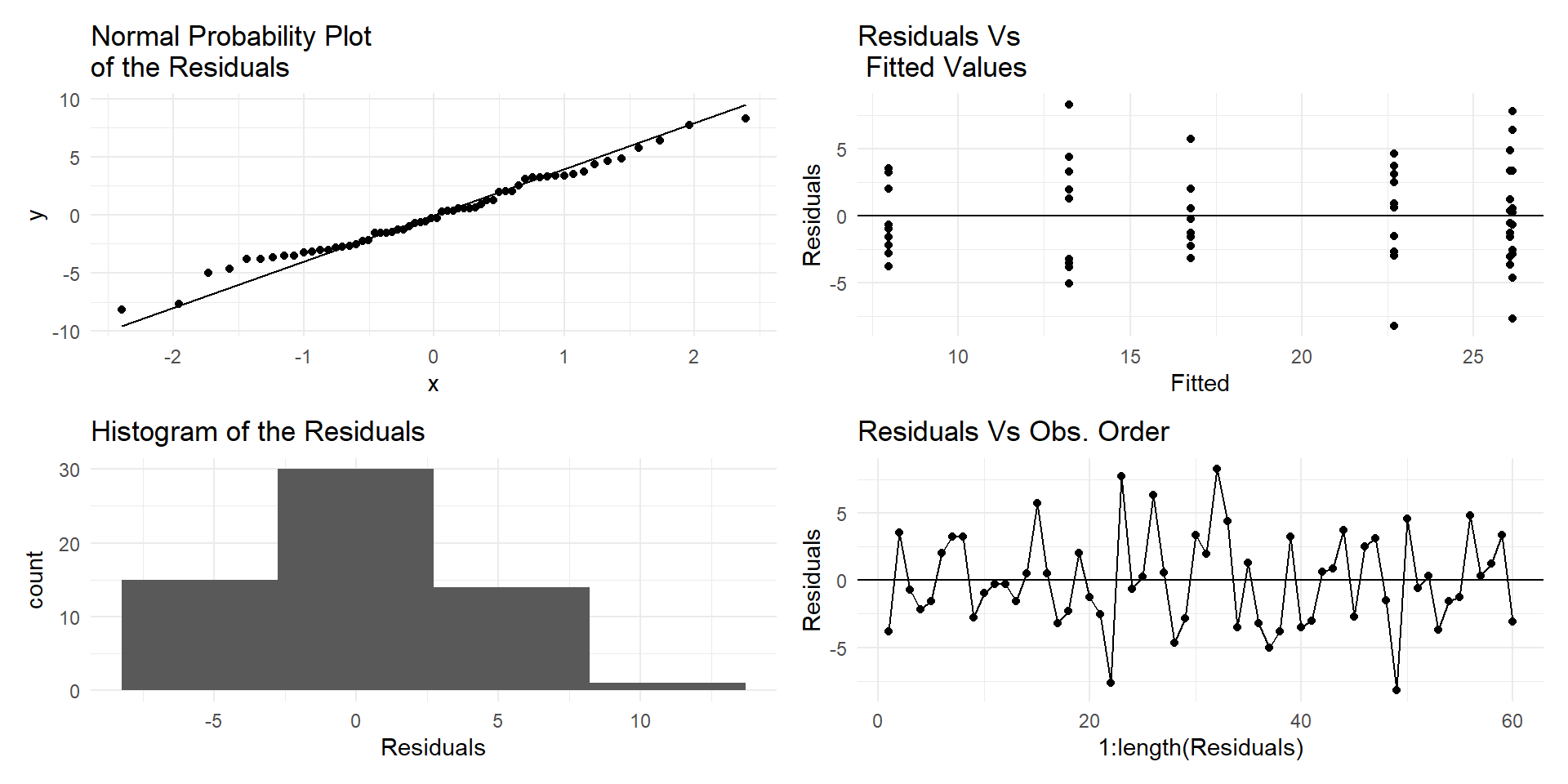
Visualize assumptions

plot(aov(burntime ~ fabric, data = fabric))

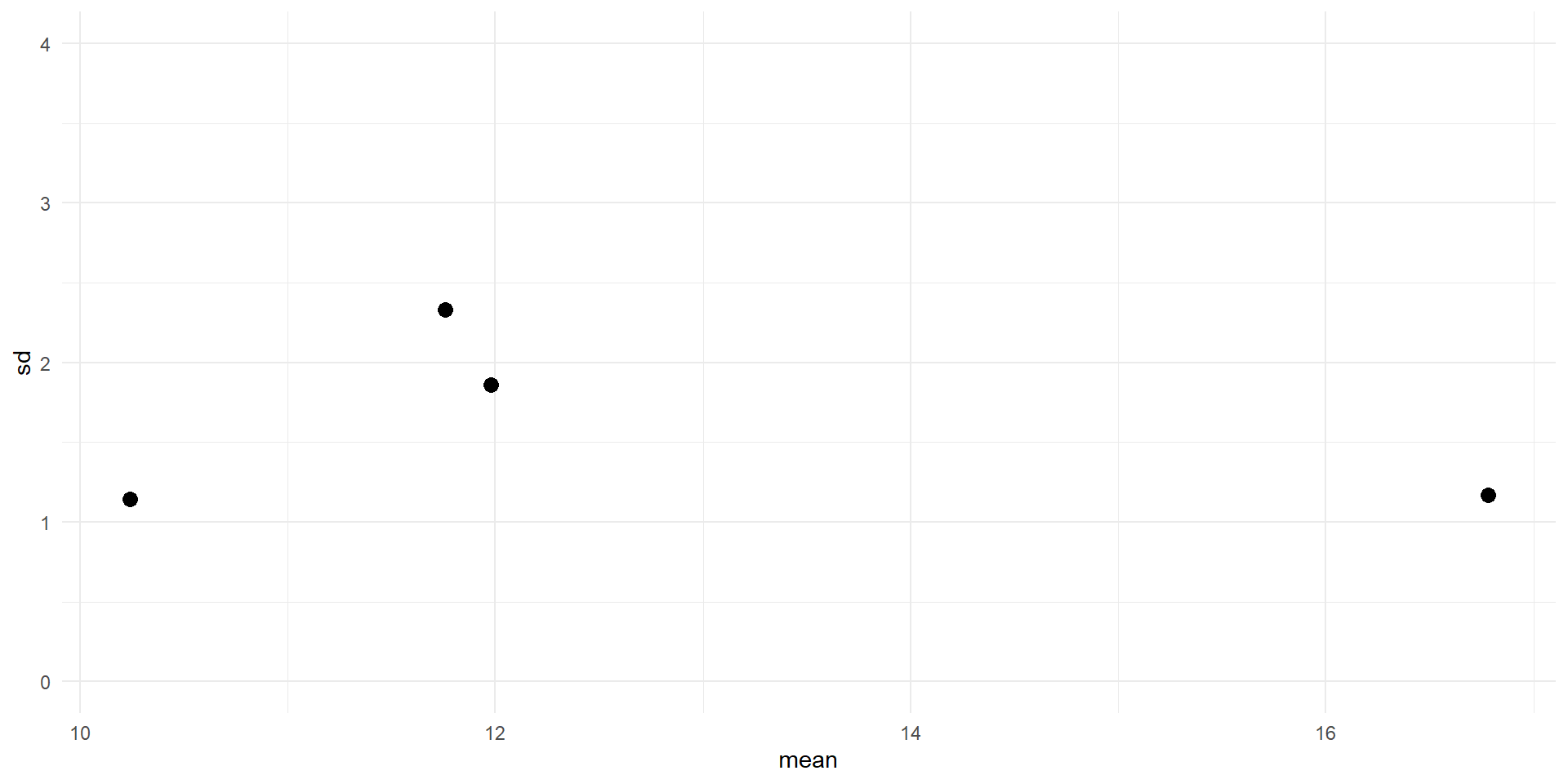
Visualize assumptions

Figure 1: SD vs mean for four fabrics

Residuals must be independent of means.
- If SD increases with mean, try square root or logarithmic transformation.

With only four fabrics in the sample, it is difficult to make any definitive claim.

If the assumptions were valid, we would expect the four points to fall approximately along a horizontal band indicating constant standard deviations, and hence variances, regardless of the means of the groups.

This figure suggests that this is the case, so the assumption of equal variances appears to be valid.

Equal variance

Bartlett’s test: - null hypothesis: equal variances - but it has an assumption of its own (response variable must be normally distributed)

Levene’s test - null hypothesis: equal variances - is applicable for any continuous distribution

bartlett.test(burntime ~ fabric, data = fabric)


    Bartlett test of homogeneity of variances

data:  burntime by fabric
Bartlett's K-squared = 2.6606, df = 3, p-value = 0.447

car::leveneTest(burntime ~ fabric, data = fabric)

Levene's Test for Homogeneity of Variance (center = median)
      Df F value Pr(>F)
group  3  0.1788 0.9092
      16

What if the equal variance assumption is violated?

ANOVA’s are considered to be fairly robust against violations of the equal variances assumption as long as each group has the same sample size.

If this assumption is violated, the most common way to deal with it is to transform the response variable using one of the three transformations:

Log Transformation: Transform the response variable from y to log(y).
Square Root Transformation: Transform the response variable from y to √y.
Cube Root Transformation: Transform the response variable from y to y1/3.

By performing these transformations, the problem of heteroscedasticity typically goes away.

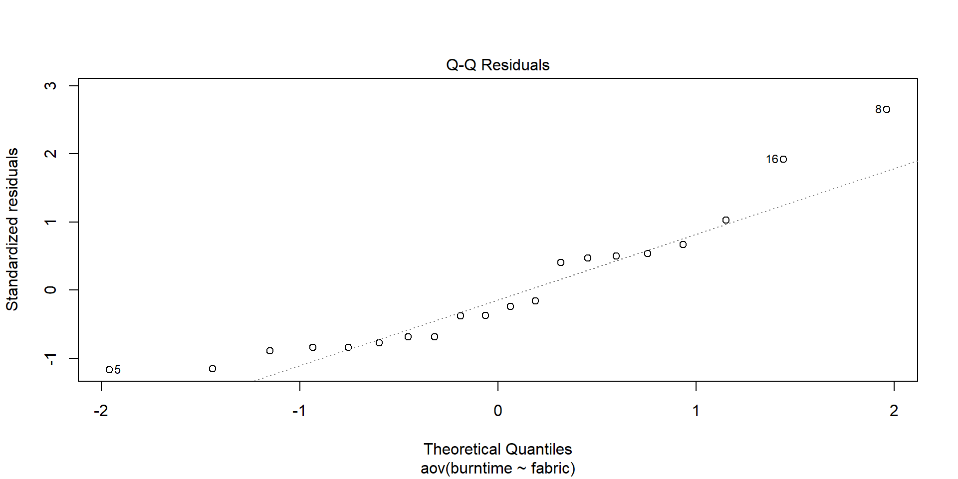
Normality

aov_fabric <- aov(burntime ~ fabric, data = fabric)
shapiro.test(aov_fabric$residuals)


    Shapiro-Wilk normality test

data:  aov_fabric$residuals
W = 0.88926, p-value = 0.02606

ANOVAs are robust to mild issues of non-normality

But if have issues with normality and unequal variance try transformations

When transformations do not help:

Weighted least squares regression: This type of regression assigns a weight to each data point based on the variance of its fitted value.
- Essentially, this gives small weights to data points that have higher variances, which shrinks their squared residuals. When the proper weights are used, this can eliminate the problem of heteroscedasticity.
Non-parametric test:
- Kruskal-Wallis Test is the non-parametric version of a one-way ANOVA

Tukey HSD

Tukey HSD (Honest Significant Differences) plot allows pairwise comparison of treatment means.
Which fabric types have different burn times? (remember the alternative hypothesis of a one-way ANOVA is at least one of the means are different)

  Tukey multiple comparisons of means
    95% family-wise confidence level

Fit: aov(formula = burntime ~ fabric, data = fabric)

$fabric
                   diff      lwr      upr     p adj
Fabric 2-Fabric 1 -5.02 -8.09676 -1.94324 0.0013227
Fabric 3-Fabric 1 -6.54 -9.61676 -3.46324 0.0000851
Fabric 4-Fabric 1 -4.80 -7.87676 -1.72324 0.0019981
Fabric 3-Fabric 2 -1.52 -4.59676  1.55676 0.5094118
Fabric 4-Fabric 2  0.22 -2.85676  3.29676 0.9968426
Fabric 4-Fabric 3  1.74 -1.33676  4.81676 0.3968476

Tukey HSD (Interval Plot)

Two way (two factor) ANOVA

Two factors are present.
A two-way ANOVA is used to estimate how the mean of a continuous variable changes according to the levels of two categorical variables.
Use a two-way ANOVA when you want to know how two independent variables, in combination, affect a dependent variable.
Very similar to multiple regression but with categorical variables.

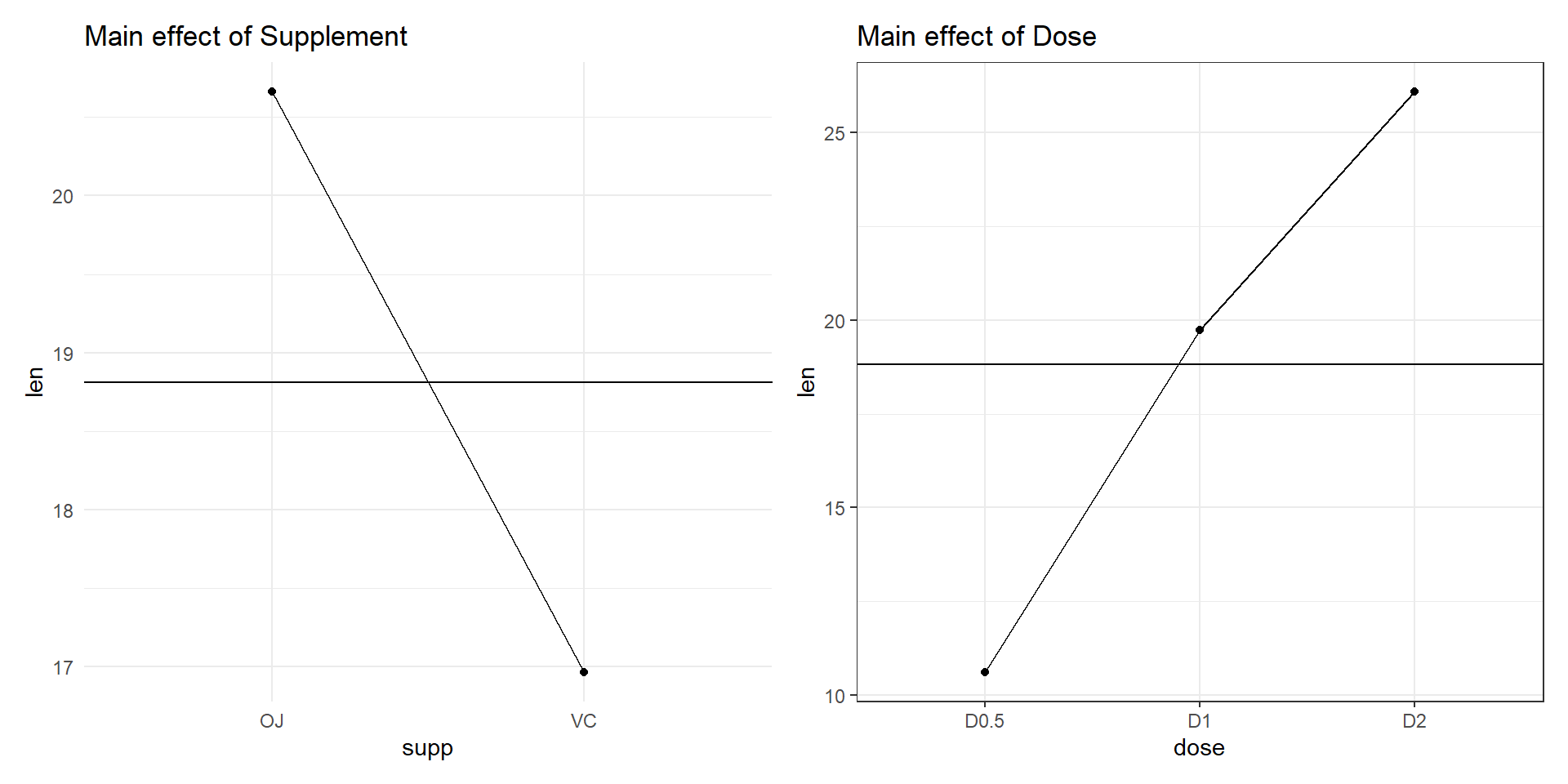
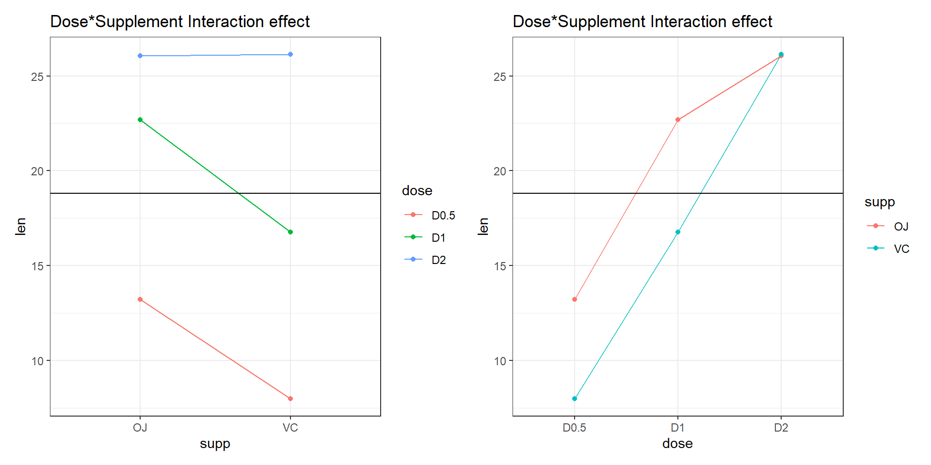
Two way (two factor) ANOVA example

Example: We will use the built in data ToothGrowth. It contains data from a study evaluating the effect of vitamin C on tooth growth in Guinea pigs. The experiment has been performed on 60 pigs, where each animal received one of three dose levels of vitamin C (0.5, 1, and 2 mg/day) by one of two delivery methods, (orange juice or ascorbic acid (a form of vitamin C and coded as VC). Tooth length was measured and a sample of the data is shown below.

   len supp dose
1  4.2   VC  0.5
2 11.5   VC  0.5
3  7.3   VC  0.5
4  5.8   VC  0.5
5  6.4   VC  0.5
6 10.0   VC  0.5

Run a Two-way ANOVA

summary(aov(len~dose+supp, data=ToothGrowth))

            Df Sum Sq Mean Sq F value   Pr(>F)    
dose         2 2426.4  1213.2   82.81  < 2e-16 ***
supp         1  205.3   205.3   14.02 0.000429 ***
Residuals   56  820.4    14.7                     
---
Signif. codes:  0 '***' 0.001 '**' 0.01 '*' 0.05 '.' 0.1 ' ' 1

A two-way ANOVA tests two null hypotheses at the same time:

All group means are equal at each level of the first variable
All group means are equal at each level of the second variable

Two-way model fit

Model:
Observation = Overall Mean + Factor 1 Effect + Factor 2 Effect + Error

\(H_0\): factor 1 means are equal; factor 2 means are equal

            Df Sum Sq Mean Sq F value   Pr(>F)    
dose         2 2426.4  1213.2   82.81  < 2e-16 ***
supp         1  205.3   205.3   14.02 0.000429 ***
Residuals   56  820.4    14.7                     
---
Signif. codes:  0 '***' 0.001 '**' 0.01 '*' 0.05 '.' 0.1 ' ' 1

Supplement and dose effects are significant at 5% level.

Main effect plots

Simply plot of response means for factor levels

Tukey HSD

teeth <- aov(len~supp+dose, data=ToothGrowth)
TukeyHSD(teeth)

  Tukey multiple comparisons of means
    95% family-wise confidence level

Fit: aov(formula = len ~ supp + dose, data = ToothGrowth)

$supp
      diff       lwr       upr     p adj
VC-OJ -3.7 -5.679762 -1.720238 0.0004293

$dose
          diff       lwr       upr p adj
D1-D0.5  9.130  6.215909 12.044091 0e+00
D2-D0.5 15.495 12.580909 18.409091 0e+00
D2-D1    6.365  3.450909  9.279091 7e-06

Summary so far

ANOVA: 1 and 2 factor
ANOVA table
Assumptions
Tukey’s HSD

Learning Objectives: Part 2

Understand the use of interactions in linear models
Use a two-way ANOVA with interactions on example data
Understand and calculate an ANOVA table when interactions are present
Describe Tukey’s post hoc tests and assumptions of ANOVAs with interactions
Understand the difference and similarities between this chapter and previous linear models covered
Review non-parametric options

Interaction effect

Whether Factor A effects are constant over Factor B effects or Factor B effects are constant over Factor A effects?
- If the answer is no, then there is an interaction between A & B.
Example:
- Temperature and pressure are factors affecting the yield in chemical experiments.
- They do interact in a mechanistic sense.

Interaction may or may not have physical meaning.

Two-way ANOVA and Interaction effects

A two-way ANOVA with interaction tests three null hypotheses at the same time:

All group means are equal at each level of the first variable
All group means are equal at each level of the second variable
There is no interaction effect between the two variables

Interaction Plots

In the absence of interaction, the plotted means of factor will be roughly parallel
- see Plot 1. A & B do not interact.
If the the plotted means of factor crossings are far from parallel, then there is interaction
- Plot 2 shows extreme (antagonistic) interaction between A & B.

Interaction Plot for Zooplankton data

library(ggplot2)
p1= ggplot(data = ToothGrowth, aes(x = supp, y = len, group=dose, colour=dose)) +
  stat_summary(fun=mean, geom="point")+
  stat_summary(fun=mean, geom="line")+
  geom_abline(intercept = mean(ToothGrowth$len), slope=0)+ 
  theme_bw()+ggtitle("Dose*Supplement Interaction effect")

p2= ggplot(data = ToothGrowth, aes(x = dose, y = len, group=supp, colour=supp)) +stat_summary(fun=mean, geom="point")+
  stat_summary(fun=mean, geom="line")+
  geom_abline(intercept = mean(ToothGrowth$len), slope=0)+ 
  theme_bw()+ggtitle("Dose*Supplement Interaction effect")
library(patchwork)
p1+p2

Interaction effect may be present

Two-way model fit

observation = mean + Factor A + Factor B + interaction effect + error

The above model is known as multiplicative model
If interaction effect is ignored, we deal with an additive model

Two-way model fit

ToothGrowth |> 
  aov(formula = len ~ supp * dose) |> 
  summary()

            Df Sum Sq Mean Sq F value   Pr(>F)    
supp         1  205.4   205.4  15.572 0.000231 ***
dose         2 2426.4  1213.2  92.000  < 2e-16 ***
supp:dose    2  108.3    54.2   4.107 0.021860 *  
Residuals   54  712.1    13.2                     
---
Signif. codes:  0 '***' 0.001 '**' 0.01 '*' 0.05 '.' 0.1 ' ' 1

Residual diagnostics

Interpreting interactions

If an interaction term is significant, the effect of Factor A depends on Factor B (and vice versa)
Use interaction plots to visualize
Posthoc tests to examine different level combinations

TukeyHSD(modl)$`supp:dose`

                 diff        lwr        upr        p adj
VC:D0.5-OJ:D0.5 -5.25 -10.048124 -0.4518762 2.425209e-02
OJ:D1-OJ:D0.5    9.47   4.671876 14.2681238 4.612304e-06
VC:D1-OJ:D0.5    3.54  -1.258124  8.3381238 2.640208e-01
OJ:D2-OJ:D0.5   12.83   8.031876 17.6281238 2.125153e-09
VC:D2-OJ:D0.5   12.91   8.111876 17.7081238 1.769939e-09
OJ:D1-VC:D0.5   14.72   9.921876 19.5181238 2.985978e-11
VC:D1-VC:D0.5    8.79   3.991876 13.5881238 2.100948e-05
OJ:D2-VC:D0.5   18.08  13.281876 22.8781238 4.855005e-13
VC:D2-VC:D0.5   18.16  13.361876 22.9581238 4.821699e-13
VC:D1-OJ:D1     -5.93 -10.728124 -1.1318762 7.393032e-03
OJ:D2-OJ:D1      3.36  -1.438124  8.1581238 3.187361e-01
VC:D2-OJ:D1      3.44  -1.358124  8.2381238 2.936430e-01
OJ:D2-VC:D1      9.29   4.491876 14.0881238 6.908163e-06
VC:D2-VC:D1      9.37   4.571876 14.1681238 5.774013e-06
VC:D2-OJ:D2      0.08  -4.718124  4.8781238 1.000000e+00

Interpreting interactions

Importance of interactions

When you have statistically significant interaction effects, you can’t interpret the main effects without considering the interactions
Interactions can be used to control for unhelpful variation (blocking effect in experiments)
Interactions can be mechanistically meaningful

ANOVA extensions and inference

Linear models can theoretically be performed with an infinite amount of predictors

The more predictors the more samples needed, your effect sample number is no longer your total sample size but the lowest treatment

Interaction effects with more than 3 (sometimes even more than 2) become very difficult to interpret and visualize

Good experimental design and causal thinking can aid in analysis design, design test then collect data, it is much harder the other way around

Indicator variables

Indicator variables are used if the predictor is qualitative rather than quantitative.
- Consider gender, a categorical variable.
  - Let \(I_1\) be an indicator variable that takes a value 1 for males and 0 for females.
  - Let \(I_2\) takes 1 for females and 0 for males.
  - Note only one of \(I_1\) & \(I_2\) is sufficient.
The minimum number of indicator variables needed is related to degrees of freedom.

ANOVA through regression

Consider the burn-time data for the four fabrics.
- The four fabric types are categorical.
- Define-
  - \(I_1\) = 1 for fabric 1 and 0 otherwise
  - \(I_2\) = 1 for fabric 2 and 0 otherwise
  - \(I_3\) = 1 for fabric 3 and 0 otherwise
  - \(I_4\) = 1 for fabric 4 and 0 otherwise
Note that any THREE indicator variables are sufficient for the four fabrics.
- 3 df for 4 fabrics

Regression summary

Regress the burn-time response on the indicator variables \(I_1\),\(I_2\), \(I_3\) & \(I_4\)

   burntime   fabric I1 I2 I3 I4
1      17.8 Fabric 1  1  0  0  0
2      16.2 Fabric 1  1  0  0  0
3      17.5 Fabric 1  1  0  0  0
4      17.4 Fabric 1  1  0  0  0
5      15.0 Fabric 1  1  0  0  0
6      11.2 Fabric 2  0  1  0  0
7      11.4 Fabric 2  0  1  0  0
8      15.8 Fabric 2  0  1  0  0
9      10.0 Fabric 2  0  1  0  0
10     10.4 Fabric 2  0  1  0  0
11     11.8 Fabric 3  0  0  1  0
12     11.0 Fabric 3  0  0  1  0
13     10.0 Fabric 3  0  0  1  0
14      9.2 Fabric 3  0  0  1  0
15      9.2 Fabric 3  0  0  1  0
16     14.9 Fabric 4  0  0  0  1
17     10.8 Fabric 4  0  0  0  1
18     12.8 Fabric 4  0  0  0  1
19     10.7 Fabric 4  0  0  0  1
20     10.7 Fabric 4  0  0  0  1

Regression and ANOVA


Call:
lm(formula = burntime ~ I1 + I2 + I3, data = fabric)

Residuals:
   Min     1Q Median     3Q    Max 
-1.780 -1.205 -0.460  0.775  4.040 

Coefficients:
            Estimate Std. Error t value Pr(>|t|)    
(Intercept)  11.9800     0.7604  15.754 3.65e-11 ***
I1            4.8000     1.0754   4.463 0.000392 ***
I2           -0.2200     1.0754  -0.205 0.840485    
I3           -1.7400     1.0754  -1.618 0.125206    
---
Signif. codes:  0 '***' 0.001 '**' 0.01 '*' 0.05 '.' 0.1 ' ' 1

Residual standard error: 1.7 on 16 degrees of freedom
Multiple R-squared:  0.7226,    Adjusted R-squared:  0.6706 
F-statistic: 13.89 on 3 and 16 DF,  p-value: 0.0001016

Compare with the one-way output

            Df Sum Sq Mean Sq F value   Pr(>F)    
fabric       3 120.50   40.17   13.89 0.000102 ***
Residuals   16  46.26    2.89                     
---
Signif. codes:  0 '***' 0.001 '**' 0.01 '*' 0.05 '.' 0.1 ' ' 1

Regression and ANOVA

fabric |> lm(formula = burntime~I1+I2+I3) |> anova()

Analysis of Variance Table

Response: burntime
          Df  Sum Sq Mean Sq F value    Pr(>F)    
I1         1 111.521 111.521 38.5718 1.248e-05 ***
I2         1   1.408   1.408  0.4871    0.4952    
I3         1   7.569   7.569  2.6179    0.1252    
Residuals 16  46.260   2.891                      
---
Signif. codes:  0 '***' 0.001 '**' 0.01 '*' 0.05 '.' 0.1 ' ' 1

Compare with the one-way output

  Tukey multiple comparisons of means
    95% family-wise confidence level

Fit: aov(formula = burntime ~ fabric, data = fabric)

$fabric
                   diff      lwr      upr     p adj
Fabric 2-Fabric 1 -5.02 -8.09676 -1.94324 0.0013227
Fabric 3-Fabric 1 -6.54 -9.61676 -3.46324 0.0000851
Fabric 4-Fabric 1 -4.80 -7.87676 -1.72324 0.0019981
Fabric 3-Fabric 2 -1.52 -4.59676  1.55676 0.5094118
Fabric 4-Fabric 2  0.22 -2.85676  3.29676 0.9968426
Fabric 4-Fabric 3  1.74 -1.33676  4.81676 0.3968476

Analysis of Covariance (ANCOVA)

Analysis of covariance (ANCOVA) is a statistical method that combines linear regression and analysis of variance (ANOVA) to evaluate the relationship between a response variable and various independent variables while controlling for covariates.

Indicator variables are used as additional regressors along with a quantitative predictor (covariate).

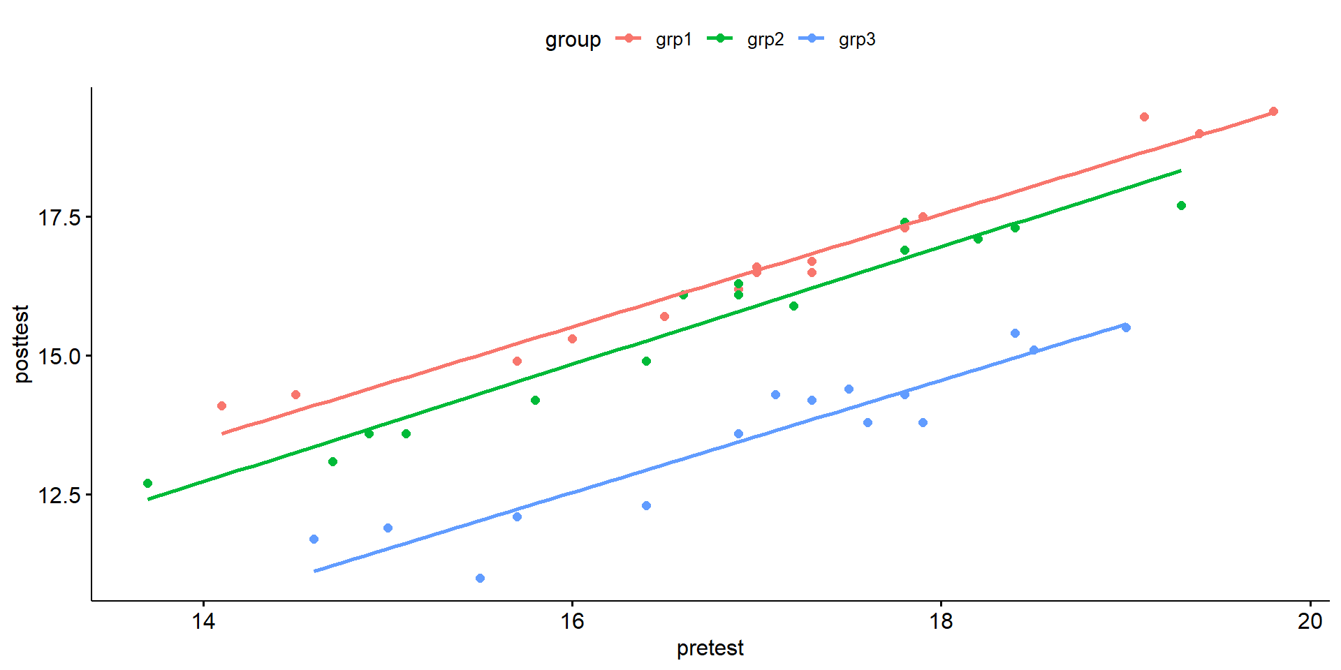
Data example: test anxiety

Researchers investigated the effect of exercises in reducing the level of anxiety, where they measured the anxiety score of three groups of individuals practicing physical exercises at different levels (grp1: low, grp2: moderate and grp3: high).

The anxiety score was measured pre- and 6-months post-exercise training programs. It is expected that any reduction in the anxiety by the exercises programs would also depend on the participant’s basal level of anxiety score.

In this analysis we use the pretest anxiety score (pretest) as the covariate and are interested in possible differences between group with respect to the post-test anxiety scores.

# A tibble: 3 × 4
  id    group pretest posttest
  <fct> <fct>   <dbl>    <dbl>
1 15    grp1     19.8     19.4
2 30    grp2     19.3     17.7
3 33    grp3     15.5     11

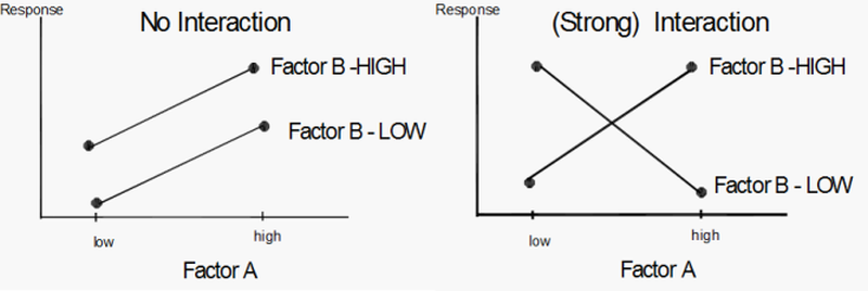
Interaction

Are the regression slopes the same?

              Df Sum Sq Mean Sq F value Pr(>F)    
group          2  72.13   36.07 203.973 <2e-16 ***
pretest        1 101.29  101.29 572.828 <2e-16 ***
group:pretest  2   0.04    0.02   0.127  0.881    
Residuals     39   6.90    0.18                   
---
Signif. codes:  0 '***' 0.001 '**' 0.01 '*' 0.05 '.' 0.1 ' ' 1

Interaction term is not significant (at sig. level of 5%).

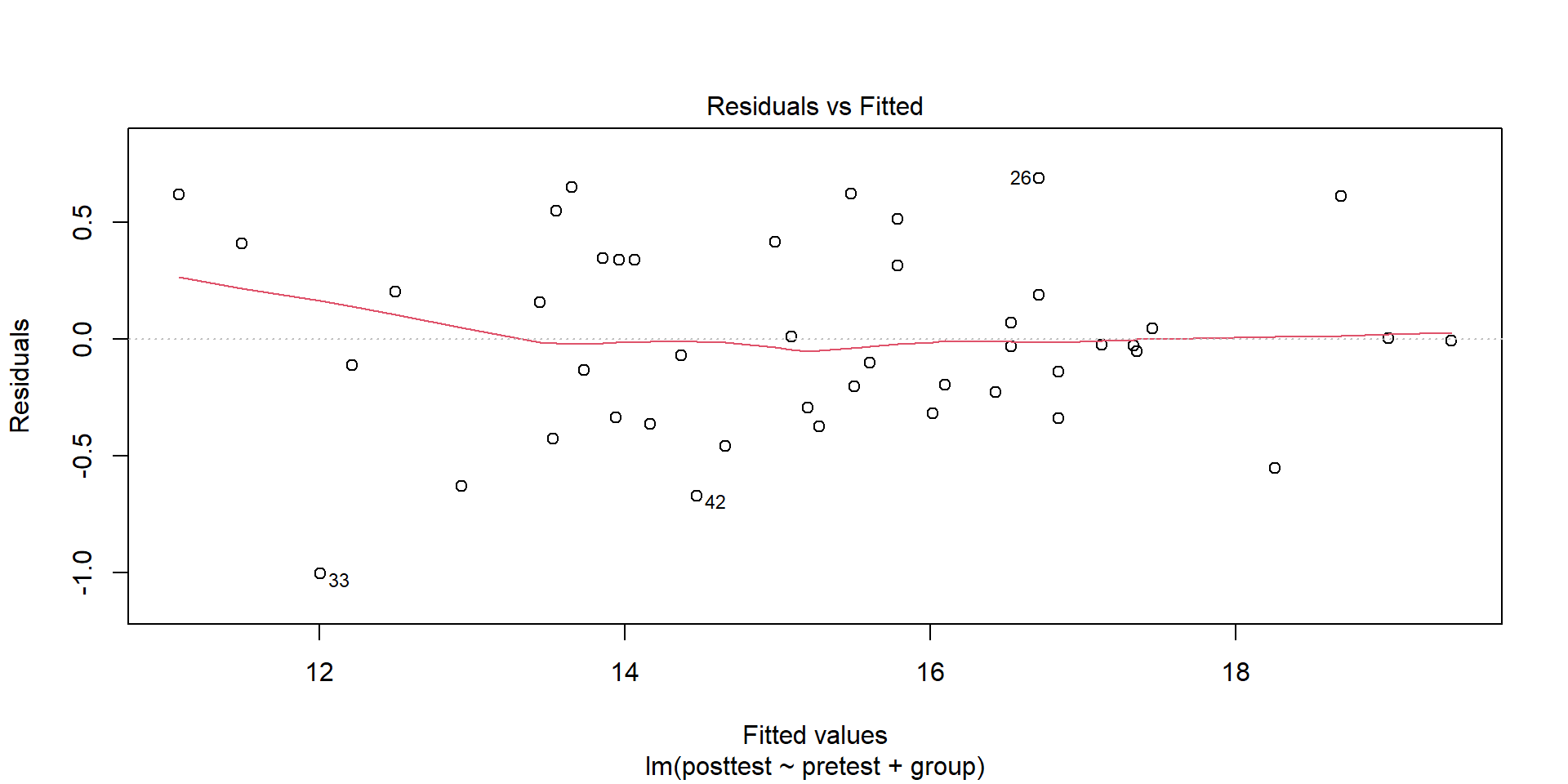
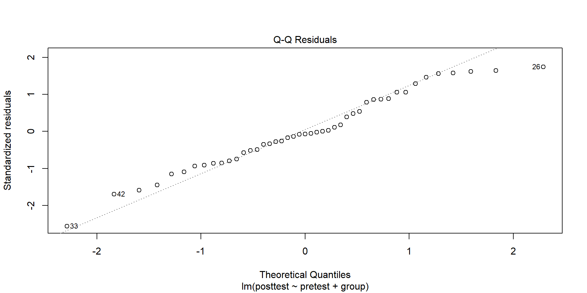
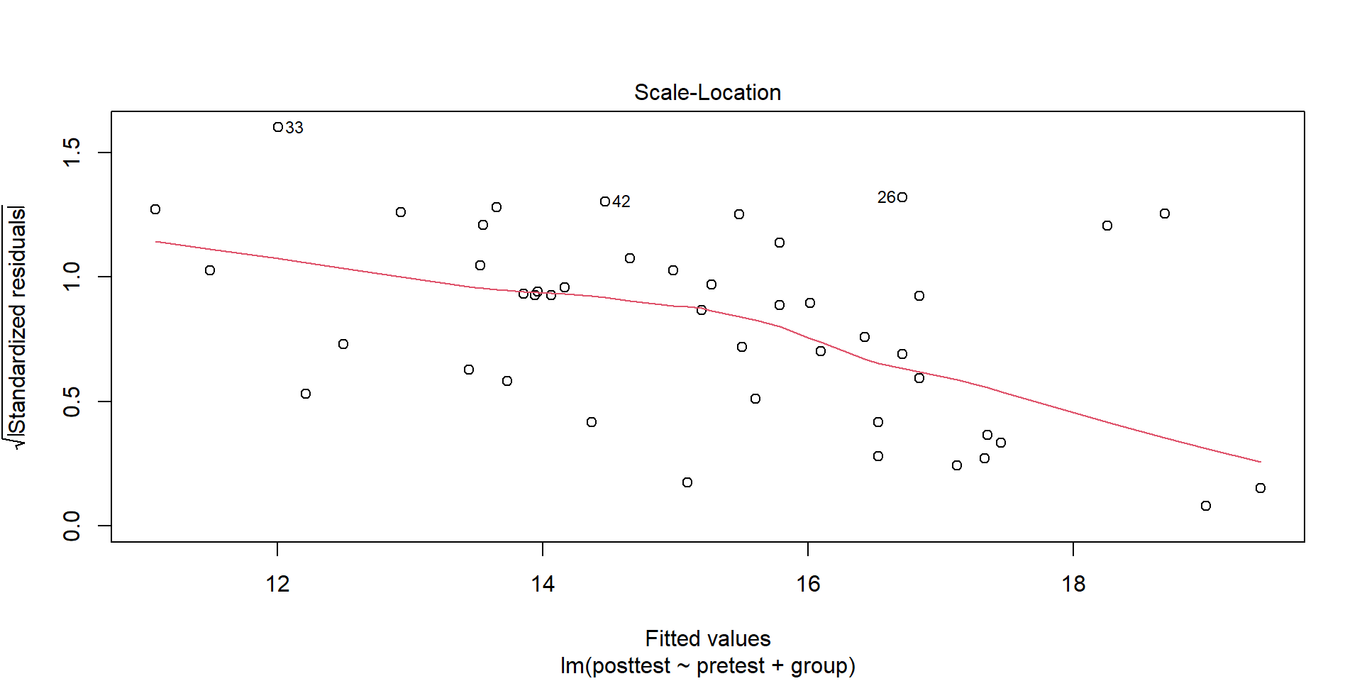
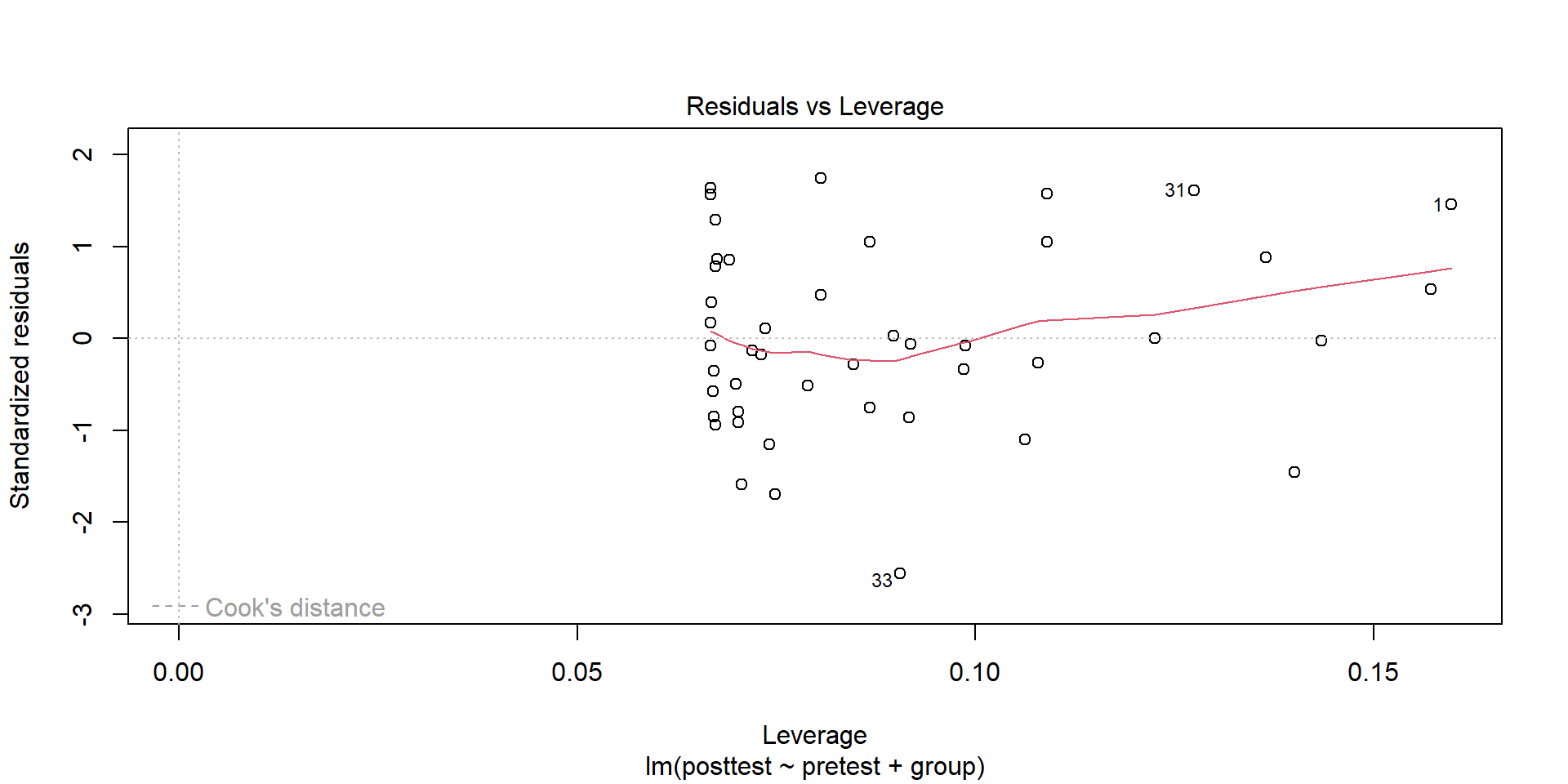
Check assumptions

Linearity:

Appears to be a linear relationship in each training group

Assumptions

Residuals:

Assumptions

Normality:

# A tibble: 1 × 3
  variable                 statistic p.value
  <chr>                        <dbl>   <dbl>
1 summary(model$residuals)     0.964   0.849

The Shapiro Wilk test was not significant (\(\alpha = 0.05\)), so we can assume normality of residuals

Equal variance:

Levene's Test for Homogeneity of Variance (center = median)
      Df F value Pr(>F)
group  2  0.2604  0.772
      42

The Levene’s test was not significant (\(\alpha = 0.05\)), so we can assume homogeneity of the residual variances for all groups.

ANCOVA fit

Estimates are the slope in each treatment (group). Remember that R assigns the first (alphabetical) level of the treatment to Intercept


Call:
lm(formula = posttest ~ pretest + group, data = anxiety)

Residuals:
     Min       1Q   Median       3Q      Max 
-1.00467 -0.29485 -0.02866  0.33846  0.68799 

Coefficients:
            Estimate Std. Error t value Pr(>|t|)    
(Intercept) -0.94088    0.72574  -1.296 0.202074    
pretest      1.02775    0.04202  24.461  < 2e-16 ***
groupgrp2   -0.64112    0.15137  -4.235 0.000126 ***
groupgrp3   -2.98463    0.15027 -19.862  < 2e-16 ***
---
Signif. codes:  0 '***' 0.001 '**' 0.01 '*' 0.05 '.' 0.1 ' ' 1

Residual standard error: 0.4114 on 41 degrees of freedom
Multiple R-squared:  0.9615,    Adjusted R-squared:  0.9587 
F-statistic: 341.5 on 3 and 41 DF,  p-value: < 2.2e-16

ANCOVA fit

Use ANOVA table to display

Analysis of Variance Table

Response: posttest
          Df Sum Sq Mean Sq F value    Pr(>F)    
pretest    1 99.400  99.400  587.16 < 2.2e-16 ***
group      2 74.023  37.011  218.63 < 2.2e-16 ***
Residuals 41  6.941   0.169                      
---
Signif. codes:  0 '***' 0.001 '**' 0.01 '*' 0.05 '.' 0.1 ' ' 1

Post-hoc tests to see which group is different

  Tukey multiple comparisons of means
    95% family-wise confidence level

Fit: aov(formula = posttest ~ group + pretest, data = anxiety)

$group
               diff       lwr        upr p adj
grp2-grp1 -1.093333 -1.458662 -0.7280048     0
grp3-grp1 -3.060000 -3.425329 -2.6946715     0
grp3-grp2 -1.966667 -2.331995 -1.6013381     0

Data example: fast-food resturants

 Restaurant  Sales Households Location I1 I2
          1 135.27        155  Highway  0  0
          2  72.74         93  Highway  0  0
          3 114.95        128  Highway  0  0
          4 102.93        114  Highway  0  0
          5 131.77        158  Highway  0  0
          6 160.91        183  Highway  0  0
          7 179.86        178     Mall  1  0
          8 220.14        215     Mall  1  0
          9 179.64        172     Mall  1  0
         10 185.92        197     Mall  1  0
         11 207.82        207     Mall  1  0
         12 113.51         95     Mall  1  0
         13 203.98        224   Street  0  1
         14 174.48        199   Street  0  1
         15 220.43        240   Street  0  1
         16  93.19        100   Street  0  1

Do we need three separate models?

ANCOVA

In order to allow for different slopes for each location, we define the product (or interaction) variables

Data set up

  Restaurant  Sales Households Location I1 I2
1          1 135.27        155  Highway  0  0
2          2  72.74         93  Highway  0  0
3          3 114.95        128  Highway  0  0
4          4 102.93        114  Highway  0  0
5          5 131.77        158  Highway  0  0
6          6 160.91        183  Highway  0  0

ANCOVA model

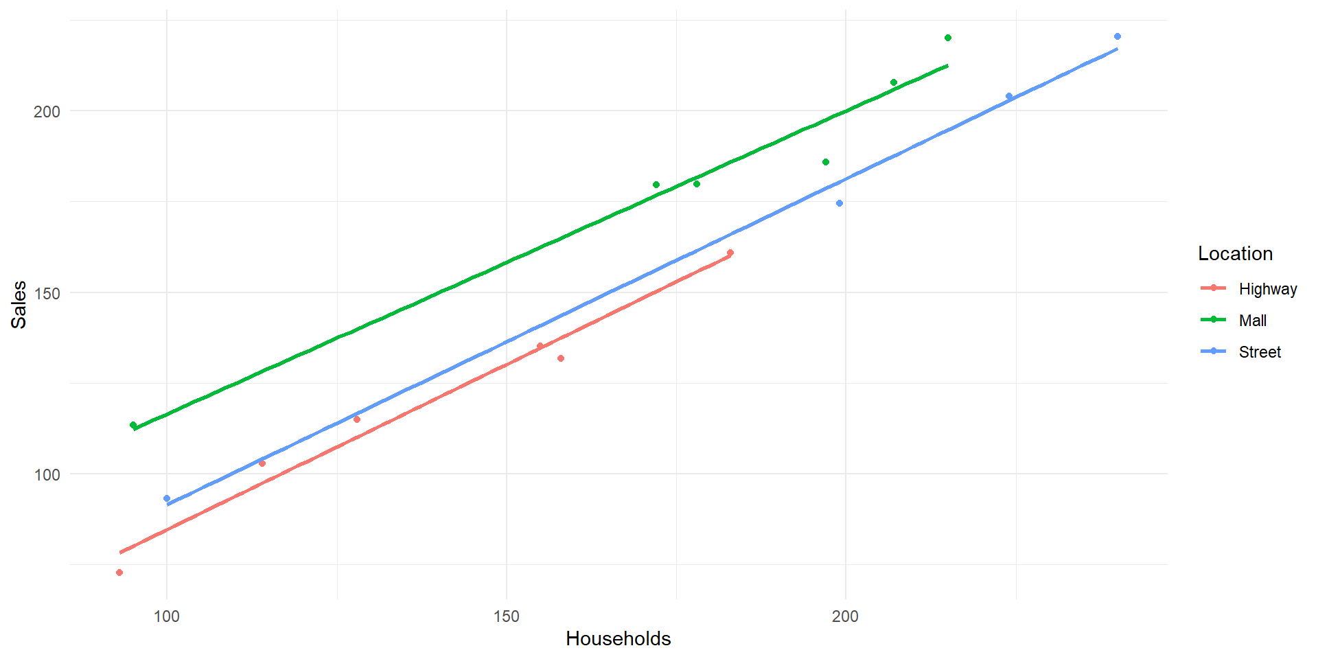
We examine the relationship between restaurant sales (response variable, in thousands of dollars) and the number of households (H) in the restaurant’s trading area and the location of the restaurant (Mall, Street, and Highway). We can use the indicator variables (\(I_1\) and \(I_2\)) to define our three locations uniquely.

\(Sales = \beta_0 + \beta_1 I_1 + \beta_2 I_2 + (\beta_3 + \beta_4 I_1 + \beta_5 I_2)Households\)

This model provides a separate model for each location as well as allows for the interaction between location of the restaurant and the number of households through the slope coefficient

ANCOVA model

\(Sales = \beta_0 + \beta_1 I_1 + \beta_2 I_2 + (\beta_3 + \beta_4 I_1 + \beta_5 I_2)Households\)

For Highway Locations: \(I_1=0\) & \(I_2=0\) hence our model simplifies to

\(Sales = \beta_{0} + (\beta_3)Households\)
For Mall Locations: \(I_1=1\) & \(I_2=0\) so the model becomes

\(Sales = \beta_{0} + \beta_{1} + (\beta_3 + \beta_4)Households\)
For Street Locations: \(I_1=0\) & \(I_2=1\) so the model becomes \(Sales = \beta_{0} + \beta_2 + (\beta_3 + \beta_5) Households\)

note R does not require us to code Location as an indicator variable

ANCOVA fit

modl = lm(Sales~Households*Location, data = restaurant)
outs <- summary(modl)$coefficients
round(outs[, 1:4], digits = 3)

                          Estimate Std. Error t value Pr(>|t|)
(Intercept)                 -6.203     11.818  -0.525    0.611
Households                   0.909      0.083  10.906    0.000
LocationMall                39.223     16.451   2.384    0.038
LocationStreet               8.036     16.273   0.494    0.632
Households:LocationMall     -0.074      0.104  -0.710    0.494
Households:LocationStreet   -0.012      0.101  -0.120    0.907

We can plug these numbers into our equations \(Sales = \beta_{0} + \beta_{1} I_1 + \beta_2 I_2 + (\beta_3 + \beta_4 I_1 + \beta_5 I_2)Households\)

\(Sales = -6.2 + 39.22 + 8.04 + ( 0.909 -0.074 -0.012) Households\)

ANCOVA model

\(Sales = -6.2 + 39.22 + 8.04 + ( 0.909 -0.074 -0.012) Households\)

For Highway Locations: \(I_1=0\) & \(I_2=0\) hence our model simplifies to

\(Sales = -6.2 + (0.909)Households\)
For Mall Locations: \(I_1=1\) & \(I_2=0\) so the model becomes

\(Sales = -6.2 + 39.22 + (0.909 -0.074)Households\)
For Street Locations: \(I_1=0\) & \(I_2=1\) so the model becomes \(Sales = -6.2 + 8.04 + (0.909 -0.012) Households\)

Graphing the model

Summary

ANOVA models study categorical predictors (factors).

-   Interaction between factors is important. 
-   ANOVA models and regression models are related and fall under a general family of linear models.

ANCOVA models employs both numerical variables (covariates) and qualitative factors for modelling.

-   Interaction between factors and covariates is important.

Review of non-parametric tests

Non-parametric tests are light on assumptions, and can be used for highly asymmetric data (as an alternative to using transformations).

Many non-parametric methods rely on replacing the observed data by their ranks.

Spearman’s Rank Correlation

Rank the \(X\) and \(Y\) variables, and then obtain usual Pearson correlation coefficient.

The plot shows non-parametric Spearman in the the upper triangle and parametric Pearson in the bottom triangle.

library(GGally)

p <- ggpairs(
  trees, 
  upper = list(continuous = wrap('cor', method = "spearman")),
  lower = list(continuous = 'cor') 
  )

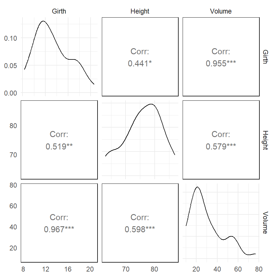
Figure 2: Comparison of Pearsonian and Spearman’s rank correlations

Wilcoxon signed rank test

A non-parametric alternative to the one-sample t-test

\(H_0: \eta=\eta_0\) where \(\eta\) (Greek letter ‘eta’) is the population median

Based on based on ranking \((|Y-\eta_0|)\), where the ranks for data with \(Y<\eta_0\) are compared to the ranks for data with \(Y>\eta_0\)

wilcox.test(tv$TELETIME, mu=1680, conf.int=T)


    Wilcoxon signed rank exact test

data:  tv$TELETIME
V = 588, p-value = 0.6108
alternative hypothesis: true location is not equal to 1680
95 percent confidence interval:
 1557.5 1906.5
sample estimates:
(pseudo)median 
          1728

t.test(tv$TELETIME, mu=1680)


    One Sample t-test

data:  tv$TELETIME
t = 0.58856, df = 45, p-value = 0.5591
alternative hypothesis: true mean is not equal to 1680
95 percent confidence interval:
 1560.633 1897.932
sample estimates:
mean of x 
 1729.283

Non-parametric ANOVA

Kruskal-Wallis test: allows to compare three or more groups

Mann-Whitney test: allows to compare 2 groups under the non-normality assumption.

Kruskal-Wallis test

The null and alternative hypotheses of the Kruskal-Wallis test are:

H0: The 3 groups are equal in terms of the variable H1: At least one group is different from the other 2 groups in terms of variable

Similar to an ANOVA the alternative hypothesis is not that all groups are different. The opposite of all groups being equal (H0) is that at least one group is different from the others (H1).

In this sense, if the null hypothesis is rejected, it means that at least one group is different from the other 2, but not necessarily that all 3 groups are different from each other. Post-hoc tests must be performed to test whether all 3 groups differ.

Mann-Whitney test

For two group comparison, pool the two group responses and then rank the pooled data

Ranks for the first group are compared to the ranks for the second group

The null hypothesis is that the two group medians are the same: \(H_0: \eta_1=\eta_2\).

load("../data/rangitikei.Rdata")
wilcox.test(rangitikei$people~rangitikei$time, conf.int=T)


    Wilcoxon rank sum test with continuity correction

data:  rangitikei$people by rangitikei$time
W = 30, p-value = 0.007711
alternative hypothesis: true location shift is not equal to 0
95 percent confidence interval:
 -88.99996 -10.00005
sample estimates:
difference in location 
             -36.46835

t.test(rangitikei$people~rangitikei$time)


    Welch Two Sample t-test

data:  rangitikei$people by rangitikei$time
t = -3.1677, df = 30.523, p-value = 0.003478
alternative hypothesis: true difference in means between group 1 and group 2 is not equal to 0
95 percent confidence interval:
 -102.28710  -22.13049
sample estimates:
mean in group 1 mean in group 2 
       22.71429        84.92308

Another form of test

kruskal.test(rangitikei$people~rangitikei$time)


    Kruskal-Wallis rank sum test

data:  rangitikei$people by rangitikei$time
Kruskal-Wallis chi-squared = 7.2171, df = 1, p-value = 0.007221

wilcox.test(rangitikei$people~rangitikei$time)


    Wilcoxon rank sum test with continuity correction

data:  rangitikei$people by rangitikei$time
W = 30, p-value = 0.007711
alternative hypothesis: true location shift is not equal to 0

Linear models Review

Family tree

T-tests, regressions, ANOVAs, and ANCOVAs are related

Similarities:

-   1 continuous response variable
-   Assumptions: normality, equal variance, and independence of residuals

Differences:

- EDA
- test statistics
- number and type of predictors

What’s the difference between a t.test and an ANOVA?

A t-test is used to determine whether or not there is a statistically significant difference between the means of two groups

sample group vs hypothetical population One-sample t-test
two independent samples Two-sample t-test
- also called independent t-test because the two samples are considered independent
samples linked in some why, not independent Paired t-test

An ANOVA is used to determine whether or not there is a statistically significant difference between the means of three or more groups, but not which group

one factor split into 3 or more groups (levels) One-way ANOVA
two factors split into 3 or more groups (levels) Two-way ANOVA
more than two factors Three factor ANOVA etc…

What’s the difference between a t.test and an ANOVA?

The main difference between a t-test and an ANOVA is in how the two tests calculate their test statistic to determine if there is a statistically significant difference between groups.

T-test:

T statistic: ratio of the mean difference between two groups relative to overal standard deviation of the differences
One-sample t-test: \(t = \frac{x-\mu}{s/\sqrt n}\)
Two-sample t-test: \(t = \frac{(\bar{x_{1}}-\bar{x_{2}})-d}{\frac{s_1}{\sqrt n} + \frac{s_2}{\sqrt n}}\)
Paired t-test: \(t=\frac{\bar{d}}{\frac{S_{d}}{\sqrt n}}\)

\(s =\) sample standard deviation \(d =\) difference

ANOVA:

F statistic: ratio of the variance between the groups relative to the variance within the groups
\(F = \frac{s_b^2}{s_w^2}\) Where \(s_b^2\) is the between sample variance, and \(s_w^2\) is the within sample variance.
MSF/MSE

When to use a t.test or an ANOVA?

In practice, when we want to compare the means of two groups, we use a t-test. When we want to compare the means of three or more groups, we use an ANOVA.

Suppose we have three groups we wish to compare the means between: group A, group B, and group C.

If you did the following t-tests:

A t-test to compare the difference in means between group A and group B
A t-test to compare the difference in means between group A and group C
A t-test to compare the difference in means between group B and group C

What if we just did many t-tests?

For each t-test there is a chance that we will commit a type I error, which is the probability that we reject the null hypothesis when it is actually true. Let’s say we set this to 0.05 (\(\alpha = 0.05\)). This means that when we perform multiple t-tests, this error rate increases.

The probability that we commit a type I error with one t-test is 1 – 0.95 = 0.05.
The probability that we commit a type I error with two t-tests is 1 – (0.95^2) = 0.0975.
The probability that we commit a type I error with three t-tests is 1 – (0.95^3) = 0.1427.

The type I error just increases!

We use a post-hoc (after) test to see which group is driving differences, these pairwise comparisons have a correction factor to adjust our Type I error

What’s the difference between a regression and an ANOVA?

A regression is used to understand the relationship between predictor variable(s) and a response variable

one predictor Simple Regression
two or more predictors Multiple Regression

An ANOVA is used to determine whether or not there is a statistically significant difference between the means of three or more groups, but not which group

one factor split into 3 or more groups (levels) One-way ANOVA
two factors split into 3 or more groups (levels) Two-way ANOVA
more than two factors Three factor ANOVA etc…

Not too much difference there

What’s the difference between a regression and an ANOVA?

Regression:

T statistic: test if each predictor’s estimate is different from 0
\(R^2\): proportion of variance explained \(\frac{SSR}{SST}\)
F statistic: overall F statistic for the regression model, \(\frac{MS_{reg}}{MS_{error}}\) where \(MS = \frac{SS}{df}\)

ANOVA:

F statistic: ratio of the variance between the groups relative to the variance within the groups
\(F = \frac{s_b^2}{s_w^2}\)

where \(s_b^2\) is the between sample variance, and \(s_w^2\) is the within sample variance.

MSF/MSE

The F statistic is the same, thats why you can produce an ANOVA table from your regression

When to use a regression or an ANOVA?

Conventionally, a regression refers to continuous predictors and ANOVAs are used for discrete variables.

BUT …

You can code discrete variable as indicator variables and then treat them as continuous and run a regression!

Generally, if you have 1 continuous and 1 discrete variable you should generate indicator variables and run a multiple regression

If you are using the continuous predictor as a covariate it would be called an ANCOVA.

You can code a discrete variable into continuous but if you do the reverse you lose statistical inference.

Reminder on Hypotheses

T-Test: difference between the means of two groups

Null: \(\mu_{1} - \mu_{2}\) is equal to \(0\) Can be \(=\), \(\le\), or \(\ge\)
Alt: \(\mu_{1} - \mu_{2}\) is not equal to \(0\) Can be \(\ne\), \(<\), or \(>\)

Regressions: understand the relationship between predictor variable(s) and a response variable

Null: true slope coefficient is \(= 0\) (i.e. no relationship)
Alt: true slope coefficient \(\ne 0\) (i.e. relationship)

ANOVA: difference between the means of three or more groups

Null: group means are equal
Alt: At least one mean is different

Where to go from here?

Linear models form the basis of a lot more statistics tests.

Chapter 8:Analysis of Variance (ANOVA) and Analysis of Covariance (ANCOVA)

Learning Objectives

ANOVA

One-way (single factor) ANOVA model

One-way ANOVA Hypotheses

One-way ANOVA

One-way (single factor) ANOVA model

ANOVA table

ANOVA table

ANOVA table

ANOVA table practice

Reminder on P values

Reminder of Sampling Distributions

Reminder of Sampling Distributions

Graphical comparison of means

One-way ANOVA model Assumptions

Visualize assumptions

Visualize assumptions

Equal variance

What if the equal variance assumption is violated?

Normality

When transformations do not help:

Tukey HSD

Tukey HSD (Interval Plot)

Two way (two factor) ANOVA

Two way (two factor) ANOVA example

Run a Two-way ANOVA

Two-way model fit

Main effect plots

Tukey HSD

Summary so far

Learning Objectives: Part 2

Interaction effect

Two-way ANOVA and Interaction effects

Interaction Plots

Interaction Plot for Zooplankton data

Two-way model fit

Two-way model fit

Residual diagnostics

Interpreting interactions

Interpreting interactions

Importance of interactions

ANOVA extensions and inference

Indicator variables

ANOVA through regression

Regression summary

Regression and ANOVA

Regression and ANOVA

Analysis of Covariance (ANCOVA)

Data example: test anxiety

Interaction

Check assumptions

Assumptions

Assumptions

ANCOVA fit

ANCOVA fit

Data example: fast-food resturants

ANCOVA

Data set up

ANCOVA model

ANCOVA model

ANCOVA fit

ANCOVA model

Graphing the model

Summary

Review of non-parametric tests

Spearman’s Rank Correlation

Wilcoxon signed rank test

Non-parametric ANOVA

Kruskal-Wallis test

Mann-Whitney test

Another form of test

Linear models Review

What’s the difference between a t.test and an ANOVA?

What’s the difference between a t.test and an ANOVA?

When to use a t.test or an ANOVA?

What if we just did many t-tests?

What’s the difference between a regression and an ANOVA?

What’s the difference between a regression and an ANOVA?

When to use a regression or an ANOVA?

Chapter 8:
Analysis of Variance (ANOVA) and Analysis of Covariance (ANCOVA)