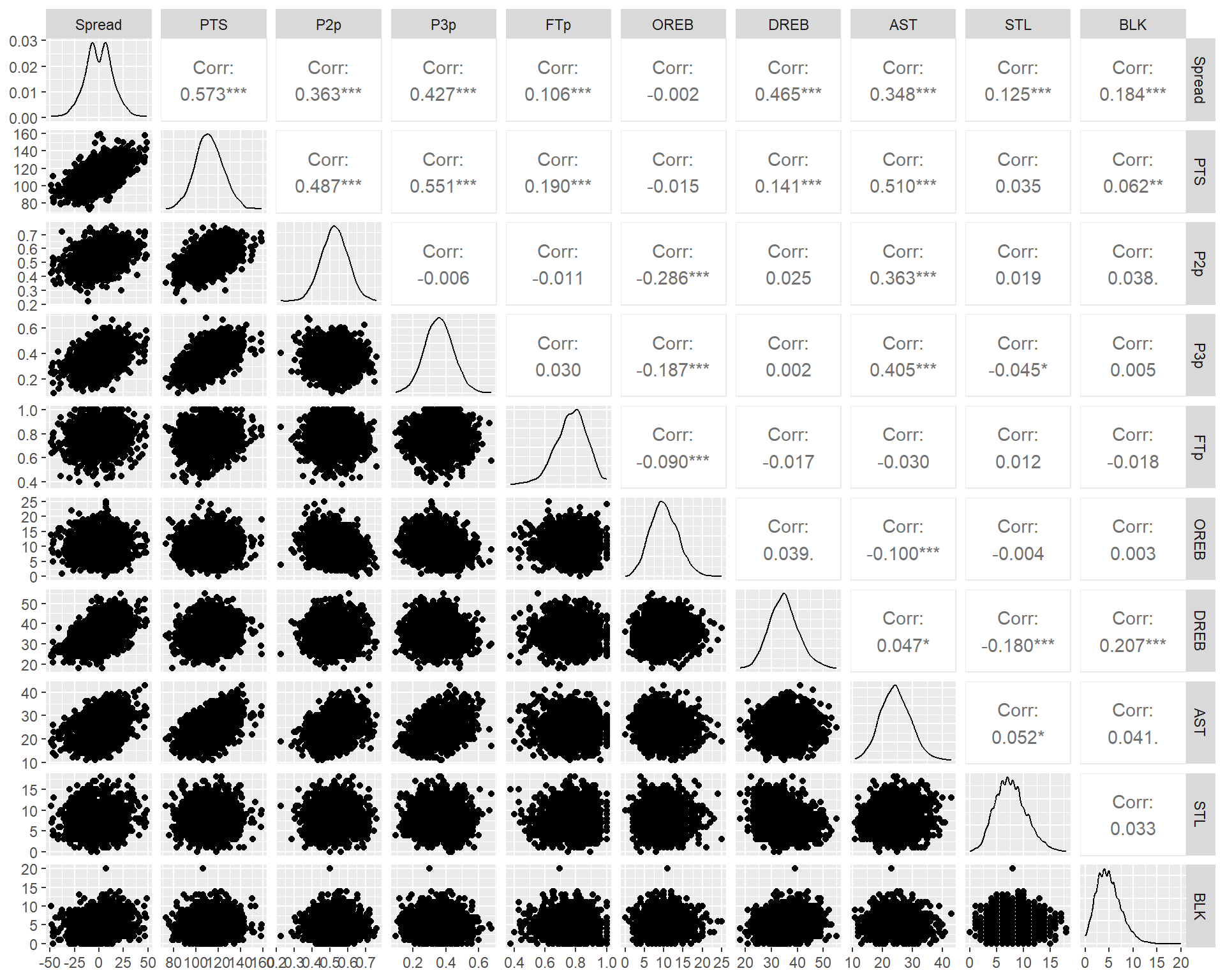
Spread: Point difference between winning and losing team PTS: Total points scored by a team in a game P2p: Percent of 2-pointers made P3p: Percent of 3-pointers made FTp: Percent of free-throws made OREB: Offensive rebounds DREB: Defensive rebounds AST: Assists STL: Steals BLK: Blocks
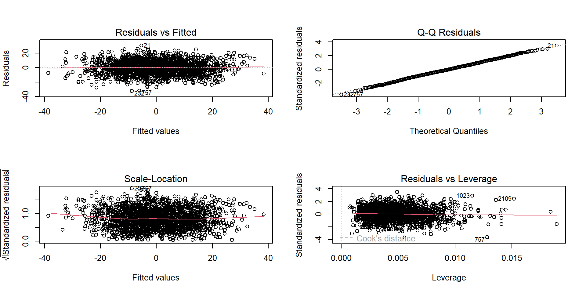
Just like with a simple regression we examine residuals to look for patterns
These look great, probably because we have a ton of data in this example.
Multicollinearity
Multicollinearity is where at least two predictor variables are highly correlated.
Multicollinearity does not affect the residual SD very much, and doesn’t pose a major problem for prediction.
The major effects of multicollinearity are:
It changes the estimates of the coefficients.
It inflates the variance of the estimates of the coefficients. That is, it increases the uncertainty about what the slope parameters are.
Therefore, it matters when testing hypotheses about the effects of specific predictors.
Multicollinearity
The impact of multicollinearity on the variance of the estimates can be quantified using the Variance Inflation Factor (VIF < 5 is considered ok).
There are several ways to deal with multicollinarity, depending on context. We can discard one of highly correlated variable, perform ridge regression, or think more carefully about how the variables relate to each other.
Multicollinearity
In R we can examine Multicollinearity using the function vif()
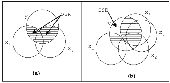
Variation in \(Y\) is separated into two parts SSR and SSE.
The shaded overlap of two circles represent the variation in \(Y\) explained by the \(X\) variables.
The total overlap of \(X_1\) and \(X_2\), and \(Y\) depends on
relationship of \(Y\) with \(X_1\) and \(X_2\)
correlation between \(X_1\) and \(X_2\)
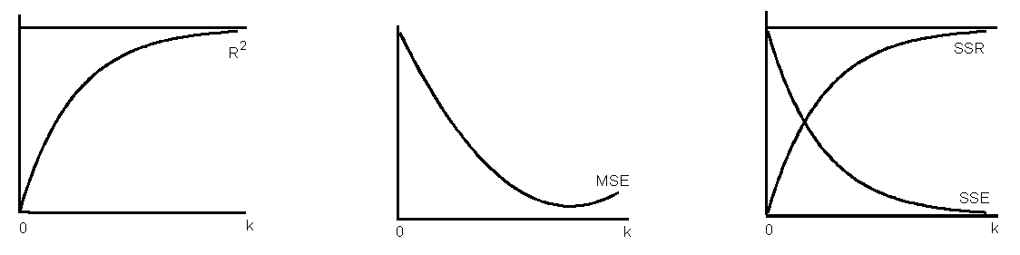
Sequential addition of predictors
Addition of variables decreases SSE and increases SSR and \(R^2\).
\(s^2\) = MSE = SSE/df decreases to a minimum and then increases since addition of variable decreases SSE but adds to df.
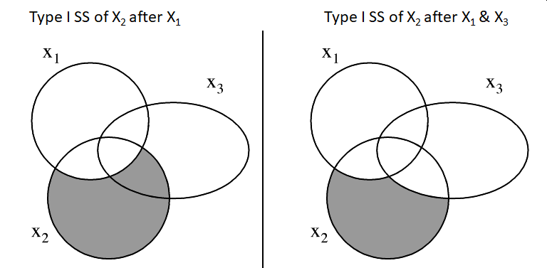
Significance of Type I or Seq.SS
The Type I SS is the SS of a predictor after adjusting for the effects of the preceding predictors in the model.
Sometimes order matters, particularly with unequal sample sizes
For unbalanced data, this approach tests for a difference in the weighted marginal means. In practical terms, this means that the results are dependent on the realized sample sizes. In other words, it is testing the first factor without controlling for the other factor, which may not be the hypothesis of interest.
F test for the significance of the additional variation explained
R function anova() calculates sequential or Type-I SS
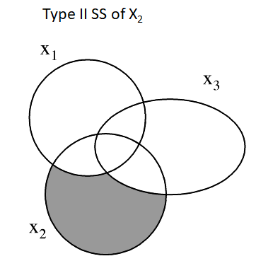
Type II
Type II SS is based on the principle of marginality.
Each variable effect is adjusted for all other appropriate effects.
equivalent to the Type I SS when the variable is the last predictor entered the model.
Order matters for Type I SS but not for Type II SS
Type III SS
Type III SS is the SS added to the regression SS after ALL other predictors including an interaction term.
This type tests for the presence of a main effect after other main effects and interaction. This approach is therefore valid in the presence of significant interactions.
If the interaction is significant SS for main effects should not be interpreted
SS types in action
Consider a model with terms A and B:
Type 1 SS:
SS(A) for factor A.
SS(B | A) for factor B.
Type 2 SS:
SS(A | B) for factor A.
SS(B | A) for factor B.
Type 3 SS:
SS(A | B, AB) for factor A.
SS(B | A, AB) for factor B.
When data are balanced and the design is simple, types I, II, and III will give the same results.
SS explained is not always a good criterion for selection of variables
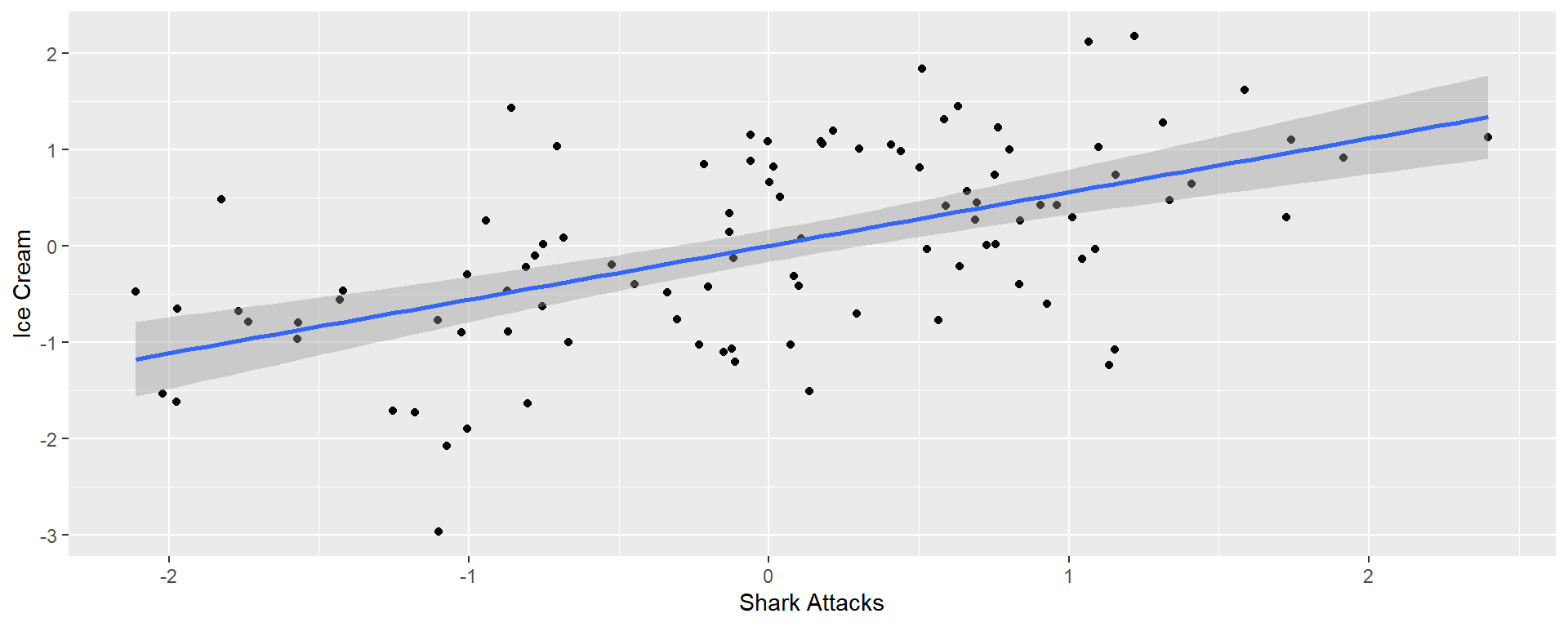
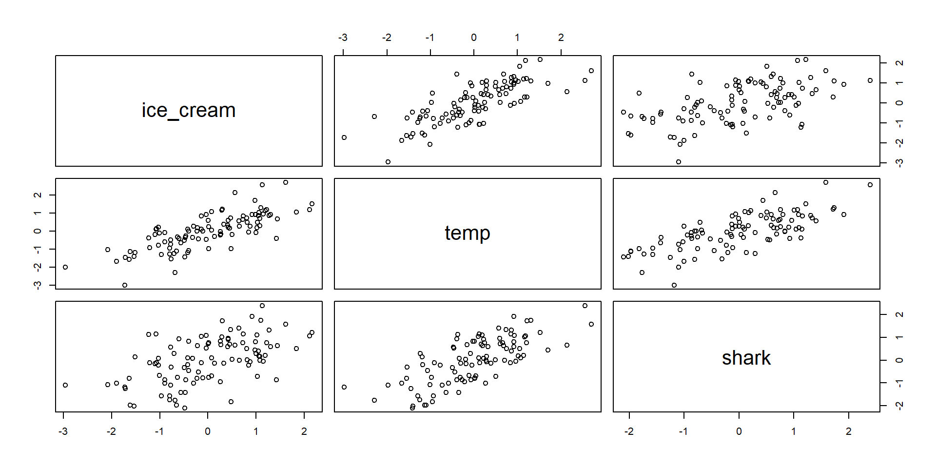
We’ll predict ice cream sales from the temperature and the number of shark attacks
First we will consider simple regressions
Single regression
Temperature Only
term
estimate
std.error
statistic
p.value
(Intercept)
0.00
0.064
0
1
temp
0.77
0.064
12
0
Shark Only
term
estimate
std.error
statistic
p.value
(Intercept)
0.000
0.083
0.00
1
shark
0.557
0.084
6.64
0
Multiple regression
Temperature Only
term
estimate
std.error
statistic
p.value
(Intercept)
0.00
0.064
0
1
temp
0.77
0.064
12
0
Shark Only
term
estimate
std.error
statistic
p.value
(Intercept)
0.000
0.083
0.00
1
shark
0.557
0.084
6.64
0
Temperature and Sharks
term
estimate
std.error
statistic
p.value
(Intercept)
0.000
0.064
0.000
1.000
temp
0.776
0.094
8.217
0.000
shark
-0.008
0.094
-0.084
0.933
Masking situation
Tend to arise when
Both predictors are associated with one another.
Have different relationships with the outcome
How do we deal with this?
Statistically there is not really an answer
The answer lies in the causes and the causes are not in the data; Shark attacks dont cause ice cream sales or vice versa
Remember that interpreting the (regression) parameter estimates always depends upon what you believe the causal model
Model Selection
The first step before selection of the best subset of predictors is to study the correlation matrix
We then perform stepwise additions (forward) or subtractions (backward) from the model and compare them
BUT…
We saw with the illustration of SS how the significance or otherwise of a variable in a multiple regression model depends on the other variables in the model
Therefore, we cannot fully rely on the t-test and discard a variable because its coefficient is insignificant
Selection of predictors
Heuristic (short-cut) procedures based on criteria such as \(F\), \(R^2_{adj}\), \(AIC\), \(C_p\) etc
Forward Selection: Add variables sequentially
convenient to obtain the simplest feasible model
Backward Elimination: Drop variables sequentially
If difference between two variables is significant but not the variables themselves, forward regression would obtain the wrong model since both may not enter the model.
Known as suppressor variables case (like masking variables discussed earlier)
Example: (try)
Call:
lm(formula = y ~ x1, data = suppressor)

Residuals:
    Min      1Q  Median      3Q     Max
-1.1691 -0.6791 -0.0033  0.6441  1.1299

Coefficients:
            Estimate Std. Error t value Pr(>|t|)
(Intercept) 11.98876    1.26689    9.46  3.4e-07 ***
x1           0.00375    0.41608    0.01     0.99
---
Signif. codes:  0 '***' 0.001 '**' 0.01 '*' 0.05 '.' 0.1 ' ' 1

Residual standard error: 0.832 on 13 degrees of freedom
Multiple R-squared:  6.24e-06,  Adjusted R-squared:  -0.0769
F-statistic: 8.11e-05 on 1 and 13 DF,  p-value: 0.993
Call:
lm(formula = y ~ x2, data = suppressor)

Residuals:
    Min      1Q  Median      3Q     Max
-1.0900 -0.6334  0.0002  0.6146  1.0403

Coefficients:
            Estimate Std. Error t value Pr(>|t|)
(Intercept)   10.632      0.811   13.11  7.2e-09 ***
x2             0.195      0.113    1.74     0.11
---
Signif. codes:  0 '***' 0.001 '**' 0.01 '*' 0.05 '.' 0.1 ' ' 1

Residual standard error: 0.75 on 13 degrees of freedom
Multiple R-squared:  0.188, Adjusted R-squared:  0.126
F-statistic: 3.02 on 1 and 13 DF,  p-value: 0.106
Call:
lm(formula = y ~ x1 + x2, data = suppressor)

Residuals:
     Min       1Q   Median       3Q      Max
-0.01363 -0.00945 -0.00228  0.00863  0.01632

Coefficients:
            Estimate Std. Error t value Pr(>|t|)
(Intercept) -4.51541    0.06114   -73.8   <2e-16 ***
x1           3.09701    0.01227   252.3   <2e-16 ***
x2           1.03186    0.00368   280.1   <2e-16 ***
---
Signif. codes:  0 '***' 0.001 '**' 0.01 '*' 0.05 '.' 0.1 ' ' 1

Residual standard error: 0.0107 on 12 degrees of freedom
Multiple R-squared:     1,  Adjusted R-squared:     1
F-statistic: 3.92e+04 on 2 and 12 DF,  p-value: <2e-16
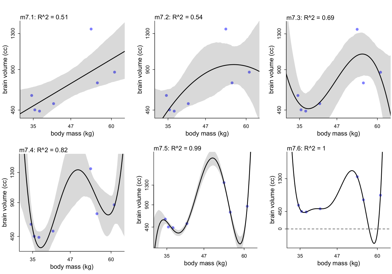
Ockham’s razor
Nunca ponenda est pluralitas sine necesitate
(Plurality should never be posited without necessity)
Problem: fit to sample always (*multi-level models can be counter-examples) improves as we add parameters.
Dangers of “stargazing”: selecting variables with low p-values (aka ‘lots of stars’). P-values are not designed to cope with over-/under-fitting.
Overfitting
Overfitting learning too much from the data, where you are almost just connecting the points rather than estimating.
Underfitting is the opposite, i.e. being insensitive to the data.
aka Models with fewer assumptions are to be preferred.
In practice, we have to choose between models that differ both in accuracy and simplicity. The razor is not really a useful guidance for this trade off.
We need tools
All possible models:
An exhaustive screening of all possible regression models can also be done using software
Best Subsets: Stop at each step and check whether predictors, in the model or outside, are the best combination for that step.
time consuming to perform when the predictor set is large
Remember permutations
For example:
If we fix the number of predictors as 3, then 20 regression models are possible
What criteria do we use?
Multiple options
- R squared
- Sums of squared (different types, for testing predictor significance)
- Information criteria (AIC, BIC etc)
- For prediction: MSD/MSE, MAD, MAPE
- \(C_p\)
Remember its about balance and what you are looking for (fit vs prediction, complexity vs generality)
Note
If a model stands out, it will perform well in terms of all summary measures.
If a model does not stand out, summary measures will contradict.
When \(R^2\) becomes absurd
Model selection
Residual SD depends on its degrees of freedom
So comparison of models based on Residual SD is not fully fair
The following three measures are popular prediction modelling and similar to residual SD
Mean Squared Deviation (MSD): mean of the squared errors (i.e., deviations) (also called MSE)
Akaike Information Criterion (AIC; smaller is better)
\[AIC = n\log \left(\frac{SSE}{n} \right) + 2p\] - Bayesian Information Criterion (BIC) places a higher penalty that depends on, the number of observations.
As a result BIC fares well for selecting a model that explains the relationships well while AIC fares well when selecting a model for prediction purposes.
Other variations: WAIC, AICc, etc (we will not cover them)
Software
In \(R\), lm() and step() function will perform the tasks
leaps() and HH packages contain additional functions
dredge() in MuMIn will produce all the subset models given a full model
Also MASS, car, caret, and SignifReg R packages
R base package step-wise selection is based on \(AIC\) only.
Cross validation (review from Chapter 6)
In sample error vs prediction error
For simpler models, increasing the number of parameters improves the fit to the sample.
But it seems to reduce the accuracy of the out-of-sample predictions.
Most accurate models trade off flexibility (complexity) and overfitting
General idea: - Leave out some observations. - Train the model on the remaining samples; score on those left out. - Average over many left-out sets to get the out-of-sample (future) accuracy.
Cross validated selection: Data example
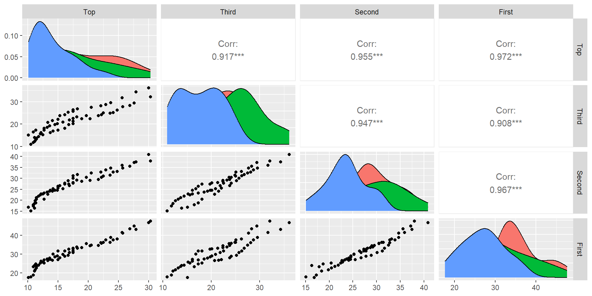
Consider the pinetree data set which contains the circumference measurements of pine trees at four positions (First is bottom)
Cross validated selection
Model selection can be done focusing on prediction
Subset selection object
3 Variables  (and intercept)
       Forced in Forced out
Third      FALSE      FALSE
Second     FALSE      FALSE
First      FALSE      FALSE
1 subsets of each size up to 2
Selection Algorithm: backward
         Third Second First
1  ( 1 ) " "   " "    "*"
2  ( 1 ) "*"   " "    "*"
Polynomial models
A polynomial model includes the square, cube of predictor variables as additional variables.
High correlation (multicollinearity) between the predictor variables may be a problem in polynomial models, but not always.
Polynomial models: Data example
We can fit a simple linear regression using the Pine tree data
pine1 <-lm(Top ~ First, data = pinetree) summary(pine1)
Call:
lm(formula = Top ~ First, data = pinetree)

Residuals:
   Min     1Q Median     3Q    Max
-2.854 -0.881 -0.195  0.630  3.176

Coefficients:
            Estimate Std. Error t value Pr(>|t|)
(Intercept)   -6.334      0.765   -8.28  2.1e-11 ***
First          0.763      0.024   31.78  < 2e-16 ***
---
Signif. codes:  0 '***' 0.001 '**' 0.01 '*' 0.05 '.' 0.1 ' ' 1

Residual standard error: 1.29 on 58 degrees of freedom
Multiple R-squared:  0.946, Adjusted R-squared:  0.945
F-statistic: 1.01e+03 on 1 and 58 DF,  p-value: <2e-16
Look closer
Looks non-linear
Polynomial models: Data example
                                  Estimate Std. Error t value Pr(>|t|)
(Intercept)                         44.121      7.039    6.27        0
poly(First, degree = 3, raw = T)1   -3.972      0.695   -5.71        0
poly(First, degree = 3, raw = T)2    0.142      0.022    6.39        0
poly(First, degree = 3, raw = T)3   -0.001      0.000   -5.95        0
```
- For the pinetree example, all the slope coefficients are highly significant for the cubic regression
- Not so for the quadratic regression
```
                                  Estimate Std. Error t value Pr(>|t|)
(Intercept)                           3.85      2.450   1.569    0.122
poly(First, degree = 2, raw = T)1     0.10      0.155   0.646    0.521
poly(First, degree = 2, raw = T)2     0.01      0.002   4.319    0.000
Raw polynomials do not preserve the coefficient estimates but orthogonal polynomials do.
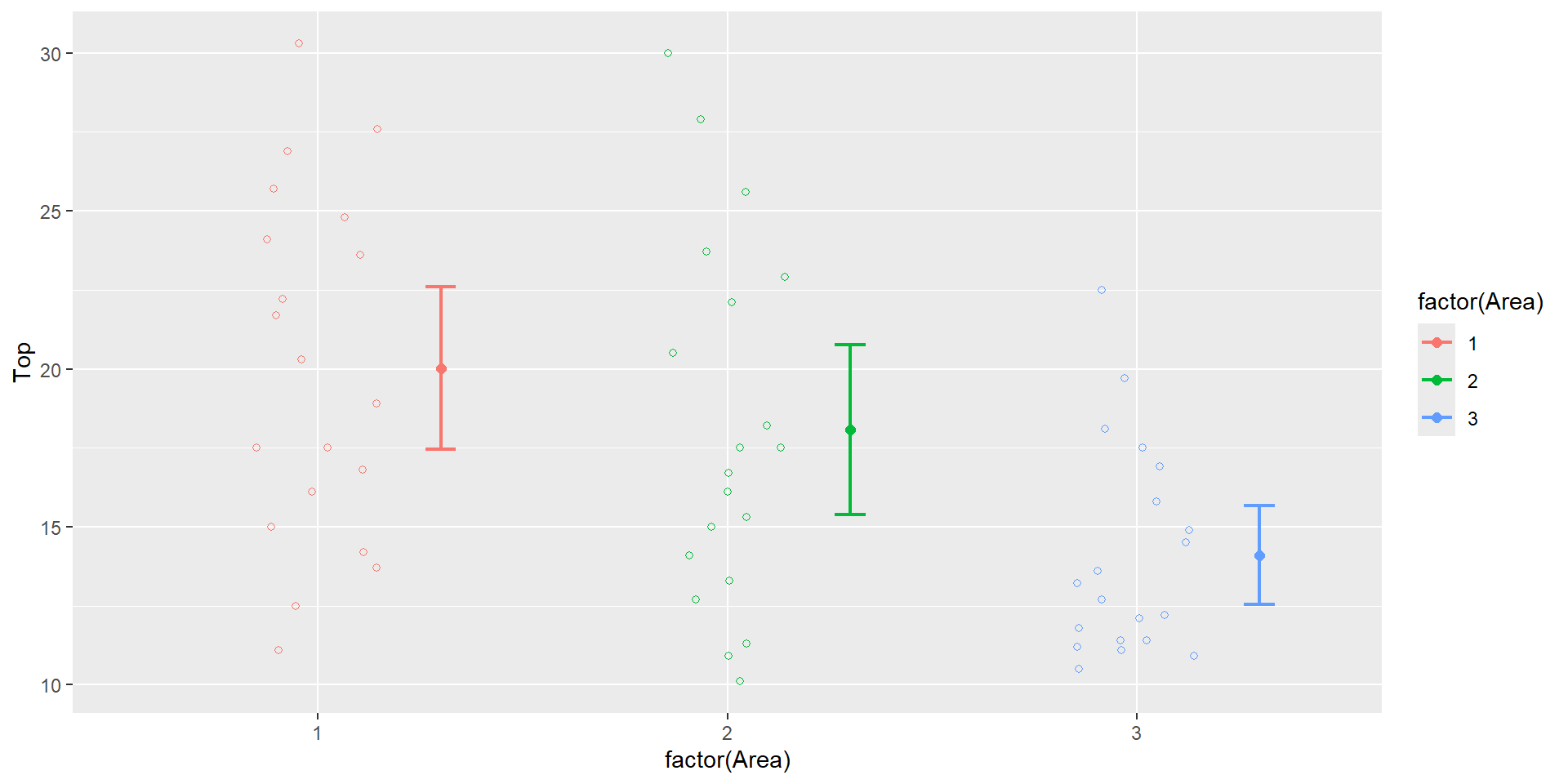
There are three different areas of the forest in the pinetree dataset. So we can define three indicator variables.
Only two indicator variables are needed because there is only 2 degrees of freedom for the 3 areas.
Regression output
Regression of Top Circumference on Area Indicator Variables
term
estimate
std.error
statistic
p.value
(Intercept)
20.02
1.11
17.98
0.00
I2
-1.96
1.57
-1.24
0.22
I3
-5.92
1.57
-3.76
0.00
The y-intercept is the mean of the response for the omitted category
20.02 is the mean Top circumference for the first Area
slopes are the difference in the mean response
-1.96 is the drop in the mean top circumference in Area 2 when compared to Area 1 (which is not a significant drop)
-5.92 is the drop in the mean top circumference in Area 3 when compared to Area 1 (which is a highly significant drop)
Analysis of Covariance model employs both numerical and categorical predictors (covered later on).
We specifically include the interaction between them
Summary
Regression methods aim to fit a model by least squares to explain the variation in the dependent variable \(Y\) by fitting explanatory \(X\) variables.
Matrix plots (EDA) and correlation coefficients provide important clues to the interrelationships.
For building a model, the additional variation explained is important. Summary criterion such as \(AIC\) is also useful.
A model is not judged as the best purely on statistical grounds.