Chapter 5:
Tabulated Counts

Analysing frequencies

• This chapter focuses on data that consist of frequencies or counts of occurrences of some events

• Wish to compare observed with what we would have expected

• We will cover the \(\chi ^ 2\) distribution, “Goodness-of-fit” tests, and test of independence

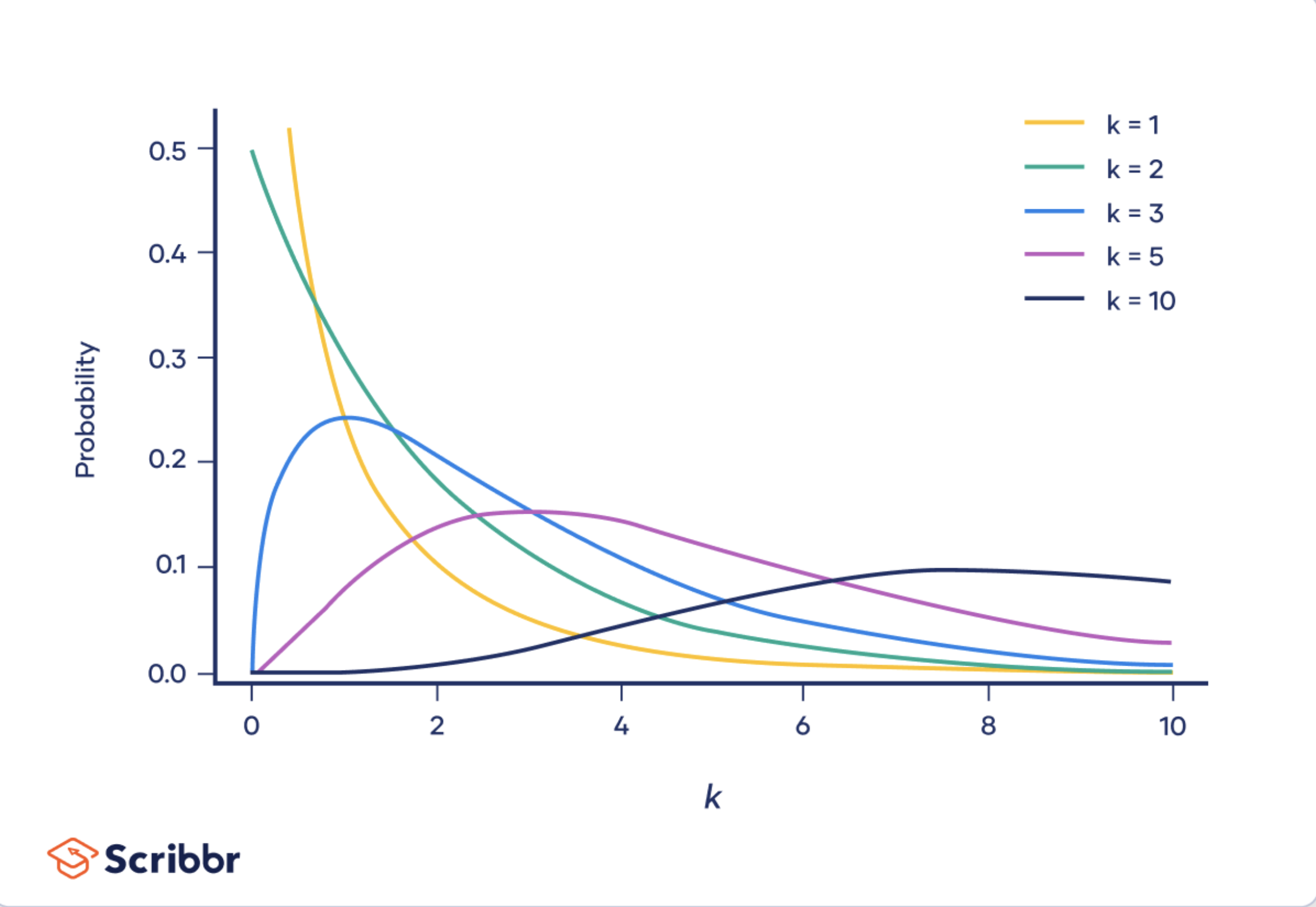
Chi squared distribution

• Continuous 0 to infinity; starts at 0 because it is a square (a square number can’t be negative)

• The mean of this distribution is its degrees of freedom (k)

• It is right skewed, mean greater than median and mode; variance is \(2k\)

• Shape of the \(\chi ^ 2\) distribution is determined by the degrees of freedom (k), at very high k (90 or greater) \(\chi ^ 2\) distribution resembles the normal distribution

• Main purpose is hypothesis testing, not describing real-world distributions

Tables and frequencies

• We often have hypotheses regarding the frequencies of levels of a factor or group of factors.

  • For a single two-level factor (e.g., male vs female, survived vs died), we might wish to know how likely the data are to have come from a population with equal proportions (or some other specified proportion).

  • For two factors, we might wish to know whether they are independent.

• In either case, we can specify a null hypothesis and test it using data.

• To do so, compare observed counts with expected counts, where the expected counts are derived from our null model about the population.

• We are employing the Chi-squared statistic with data which consists of integers. That is, the data are discrete rather than continuous.

Examples of data with one factor

Example 1

• A dataset contains 40 males and 50 females.
• How plausible is the null model of these counts coming from a population with 50% males and 50% females?
• The expected counts in this case would be 45 males and 45 females.

Examples of data with one factor

Example 2

• Does the distribution of rejects of metal castings by causes in a particular week vary from the long-term average counts?
• Treat the long-term average counts as the expected counts.
• Compare observed counts with expected counts.

Causes of rejection	Rejects during the week	Long-term average
sand	90	82
misrun	8	4
shift	16	10
drop-	8	6
corebreak	23	21
broken	21	20
other	5	8

Chi-squared test statistic

\[ \chi ^{2} =\sum _{1}^{c}\frac{\left({\rm Observed-Expected}\right)^{{\rm 2}} }{{\rm Expected}} =\sum _{1}^{c}\frac{\left( O-E\right)^{2}}{E} \]

If the number of categories is \(c\), then the degrees of freedom is \(c-1\).

Chi-squared test statistic

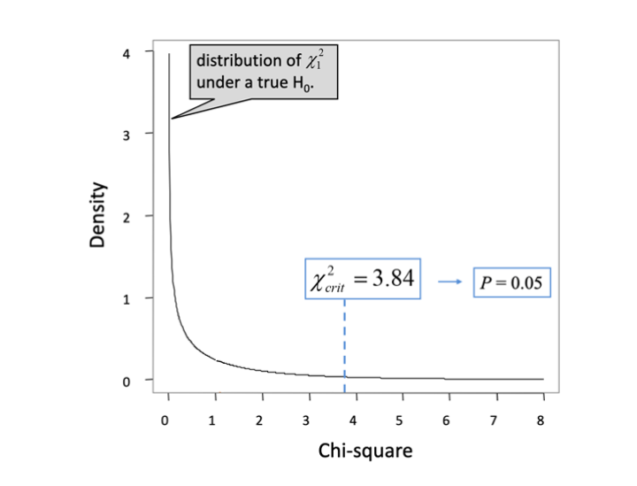
If the null hypothesis were true, then the value of \(\chi ^{2}\) calculated from our data is a random value from a Chi-squared distribuion: \[ \chi_{0} ^{2} = \chi_{c-1} ^{2} \] Once we calculate the test statistic, we can compare our observed value with its distribution under \(H_{0}\) to calculate a p-value.

Assumptions

• The classification of observations into groups must be independent

• No more than 20% of categories should have expected counts less than 5

Goodness of fit test

• Compare observed frequencies with expected frequencies under some specified null hypothesis.

• Make a hypothesis about the population, what would we expect the frequency to be under that hypothesis?

• For example:

  • Wish to compare the frequency of occurence of different phenotypes in an organism with the frequencies we would expect under Mendel’s laws of inheritance.
  • Wish to compare the distribution of a observation with expected count we would obtain from a Poisson distribution.

Hypotheses of this sort can be tested using the Chi-squared test statistic (\(\chi ^ 2\) = Ki Sq.)

Example

A survey of voters included 550 males and 450 females. Will you call this survey as a biased one?

Here the null hypothesis is that the ratio of males to females is 1:1.

Equivalent: the proportion of males is equal to the proportion of female in the population

Gender	\(O\)	\(E\)	\((O-E)^2/E\)
male	550	500	\((550-500)^2/ 500=5\)
female	450	500	\((450-500)^2/ 500=5\)
sum	1000	1000	10

\[ \chi ^{2} = \sum _{1}^{c}\frac{\left( O-E\right)^{2}}{E} = \frac{(550-500)^2}{500} + \frac{(450-500)^2}{500} = 10 \]

Example

• df= (2-1)=1
• At 5% level (\(\alpha =0.05\)), the critical value is only 3.84. So the sample is a biased one.

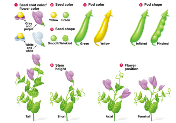
Mendel’s experiment (see Study Guide)

• Mendel discovered the principles of heredity by breeding garden peas. In one Mendel’s trials ratios of various types of peas (dihybrid-crosses) were 9:3:3:1

• The observed results are very close to expected results. This results in a small chi squared value. Were experimental results fudged or was there a confirmation bias?

Goodness of fit for distributions

• Treat class intervals as categories and obtain the actual counts (O)
• The assumed distribution gives the expected counts (E)
• Perform a goodness of fit and validate the assumed theoretical distribution
• Adjust the degrees of freedom (df) for the number of estimated parameters of the theoretical distribution
  • For example, assume that you have 10 class intervals and test for normal distribution, which has 2 parameters.
    
  • So the df for this test will be 10-1-2=7.

Goodness of fit for distributions example

A safety inspector monitors car accidents at a bustling intersection. The inspector enters the counts of monthly accidents.

Null: The sample data follow the Poisson distribution. Alternative: The sample data do not follow the Poisson distribution.

Note The Poisson distribution is a discrete probability distribution (integers) that can model counts of events or attributes in a fixed observation space. Many but not all count processes follow this distribution.

Goodness of fit for distributions example

Accidents	\(O\)	\(E\)	\((O-E)^2/E\)
0	7
1	8
2	13
3	10
>=4	12
Sum	40

Conclusion:

Tests of Independence

• In some cases, we have counts of observations cross-classified in terms of two factors.

• We are generally interested in determining whether or not the two factors are independent.

• If we consider the observations falling into each category for factor 1, is this distribution consistent across all levels of factor 2? (or vice versa)

Contingency table

• Given a two way table of frequency counts, we test whether the row and column variables are independent

• Hypotheses:

  • Null: the two factors are independent
  • written another way: the row (or column) distributions are the same

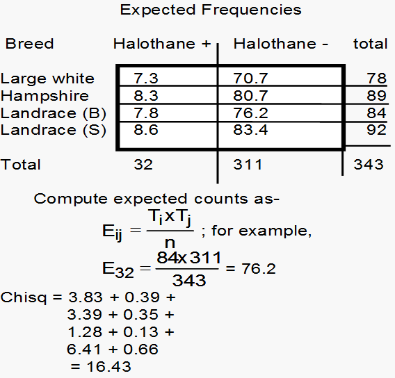
• The expected count for cell \((i,j)\) is given by \(E_{ij}\) = \((T_i \times T_j)/n\) where
  \(~~~~~T_i\), the total for row \(i\);
  \(~~~~~T_j\), the total for column \(j\)
  \(~~~~~n\), the overall total count

• Test statistic : \(\chi ^{2} =\sum _{{i=1}}^{r}\sum _{{j=1}}^{{\rm c}}\frac{\left({ O}_{{ ij}} { -E}_{{ij}} \right)^{{ 2}} }{{ E}_{{ij}} }.\)

• degrees of freedom: \((r-1)(c-1)\)

Example

Context: Porcine Stress Syndrome (PSS) result in pale, soft meat in pigs and under conditions of stress- death.

• Presence of PPS is a positive reaction to breathing halothane.
  • Selective breeding for reducing incidence of PSS

Porcine Stress Syndrome (PSS) data

	Halothane.positive	Halothane.negative	Totals
Large White	2	76	78
Hampshire	3	86	89
Landrace(B)	11	73	84
Landrace(S)	16	76	92
Totals	32	311	343

Example

Porcine Stress Syndrome (PSS) data

	Halothane.positive	Halothane.negative	Totals
Large White	2	76	78
Hampshire	3	86	89
Landrace(B)	11	73	84
Landrace(S)	16	76	92
Totals	32	311	343

chisq.test(dt)

    Pearson's Chi-squared test

data:  dt
X-squared = 16.433, df = 8, p-value = 0.03659

Computations

Porcine Stress Syndrome (PSS) data

	Halothane.positive	Halothane.negative	Totals
Large White	2	76	78
Hampshire	3	86	89
Landrace(B)	11	73	84
Landrace(S)	16	76	92
Totals	32	311	343

Inference

• The tabulated Chisq with (4-1)x(2-1) = 3 d.f are
  • 7.81 at 5% level; 16.27 at 1% level.

• Conclusion: There is a statistical evidence that the breed is not independent of the result of the Halothane test.

  • Note that large counts in the second column (Halothane negative) lead to large expected values but low contributions to chi-squared statistic.
  • This is because of the division by the appropriate expected value. On the other hand, the small observations of first column lead to small expected values but large contributions to the \(\chi ^{2}\).

Significant cell contribution

• Counts follow Poisson distribution for which mean = variance

• Hence \(\chi^{2}=\sum \frac{\left({\rm residual}\right)^{{\rm 2}} }{{\rm variance}} =\sum \left(\frac{{\rm residual}}{{\rm std\; dev}} \right)^{2}.\)

• Individual cell contribution is similar to standardized residual. Any standardized residual greater than 2 is regarded as significant.

• So \(2^2 = 4\) is treated as a significant contribution to the \(\chi ^{2}\) statistic.

Warnings

• Use only frequency counts. Use of percentages in place of counts may lead to incorrect conclusions.

• Check for small expected values. An expected value of less than 5 may lead to concern and a very small value of less than 1 is a warning. Sometimes, you can merge/combine categories in case of small expected counts.

• If the chi-squared statistic is small enough to be not significant, there is no problem.

• If chi-squared statistic is significant, check the contributions to each cell. If cells with large expected value (>5) contribute a large amount to chi-squared statistic, again there is no problem.

• If cells with expected values less than 5 lead large contributions to chi-squared statistic, the significance of the chi-squared statistic should be treated with caution.

Simpson’s paradox

Group 1

     [,1] [,2]
[1,]   80  120
[2,]   30   80

    Pearson's Chi-squared test with Yates' continuity correction

data:  group1
X-squared = 4.4809, df = 1, p-value = 0.03428

Group 2

     [,1] [,2]
[1,]   20   75
[2,]   25   20

    Pearson's Chi-squared test with Yates' continuity correction

data:  group2
X-squared = 15.122, df = 1, p-value = 0.0001008

After amalgamation of both groups

     [,1] [,2]
[1,]  100  195
[2,]   55  100

    Pearson's Chi-squared test with Yates' continuity correction

data:  all
X-squared = 0.053808, df = 1, p-value = 0.8166

Permutation test

This test is done maintaining the marginal totals.

Data: Smoking Status vs. Staff  Groupings

Smoking Status vis-a-vis Staff Groupings

	None	Moderate	Heavy	Totals
Junior employees	18	57	13	88
Junior managers	4	10	4	18
Secretaries	10	13	2	25
Senior employees	25	22	4	51
Senior managers	4	5	2	11
Totals	61	107	25	193

Permutation test

set.seed(12321)
chisq.test(tabledata, simulate.p.value = TRUE)

    Pearson's Chi-squared test with simulated p-value (based on 2000
    replicates)

data:  tabledata
X-squared = 15.672, df = NA, p-value = 0.04948

Regular Chi-square test

chisq.test(tabledata)

    Pearson's Chi-squared test

data:  tabledata
X-squared = 15.672, df = 8, p-value = 0.04733

Correspondence Analysis

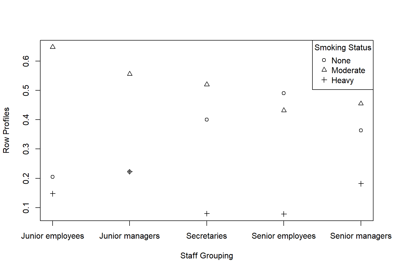
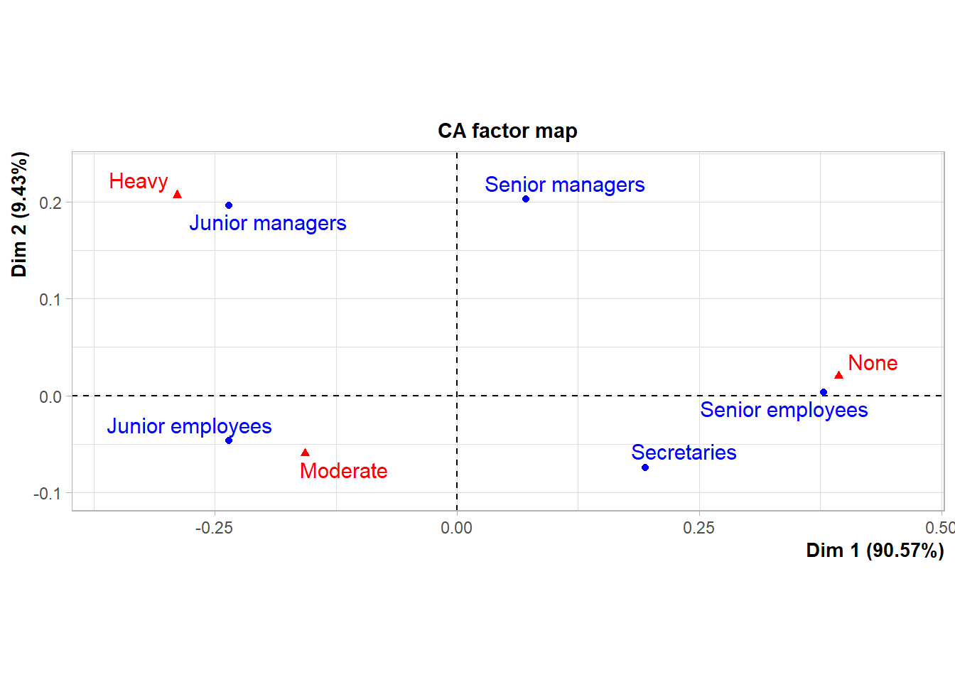
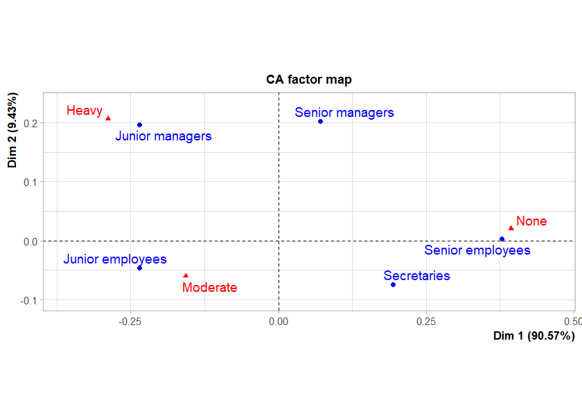
Correspondence Analysis is an exploratory statistical technique for assessing the interdependence of categorical variables whose data are presented primarily in the form of a two-way table of frequencies

Data: Smoking Status vs. Staff Groupings

                 None Moderate Heavy
Junior employees   18       57    13
Junior managers     4       10     4
Secretaries        10       13     2
Senior employees   25       22     4
Senior managers     4        5     2

    Pearson's Chi-squared test

data:  tabledata
X-squared = 15.672, df = 8, p-value = 0.04733

Row mass & row profiles

• row profiles are found dividing the cell counts by the corresponding row total

• row mass is found dividing the row totals by the grand total

                  None Moderate  Heavy
Junior employees 0.205    0.648 0.1477
Junior managers  0.222    0.556 0.2222
Secretaries      0.400    0.520 0.0800
Senior employees 0.490    0.431 0.0784
Senior managers  0.364    0.455 0.1818
rowmass          0.316    0.554 0.1295

• Similarly column profiles & column masses can be found

Graphical display of row profiles

• No clear patterns seen

Symmetric plots to find subgrouping

library("FactoMineR")
CA(tabledata) |> summary()

Call:
CA(X = tabledata) 

The chi square of independence between the two variables is equal to 15.7 (p-value =  0.0473 ).

Eigenvalues
                       Dim.1   Dim.2
Variance               0.074   0.008
% of var.             90.570   9.430
Cumulative % of var.  90.570 100.000

Rows
                   Iner*1000    Dim.1    ctr   cos2    Dim.2    ctr   cos2  
Junior employees |    26.268 | -0.235 34.372  0.962 | -0.047 12.934  0.038 |
Junior managers  |     8.784 | -0.236  7.042  0.590 |  0.197 47.082  0.410 |
Secretaries      |     5.618 |  0.195  6.670  0.873 | -0.074  9.301  0.127 |
Senior employees |    37.894 |  0.379 51.521  1.000 |  0.004  0.045  0.000 |
Senior managers  |     2.636 |  0.071  0.394  0.110 |  0.203 30.638  0.890 |

Columns
                   Iner*1000    Dim.1    ctr   cos2    Dim.2    ctr   cos2  
None             |    49.186 |  0.394 66.705  0.997 |  0.020  1.688  0.003 |
Moderate         |    15.679 | -0.157 18.619  0.873 | -0.060 25.941  0.127 |
Heavy            |    16.335 | -0.289 14.676  0.661 |  0.207 72.371  0.339 |

Symmetric plots to find subgrouping

Summary

• Goodness of fit is for testing whether the observed counts are from the hypothesised population groups.

  • For \(c\) categories (groups), the test involves \(c-1\) df.

• Contingency Table (\(r\) rows and \(c\) columns) data are tested for the independence.

  • For \(r\times c\) cells the test involves \((r-1)(c-1)\) df

• \(\chi ^{2}\) test works well if \(E> 5\). Some could be as low as 1.

• Do correspondence analysis (symmetric plots) when independence is rejected.