“A statistical analysis, properly conducted, is a delicate dissection of uncertainties, a surgery of suppositions.”
— M.J. Moroney
Statistical Inference
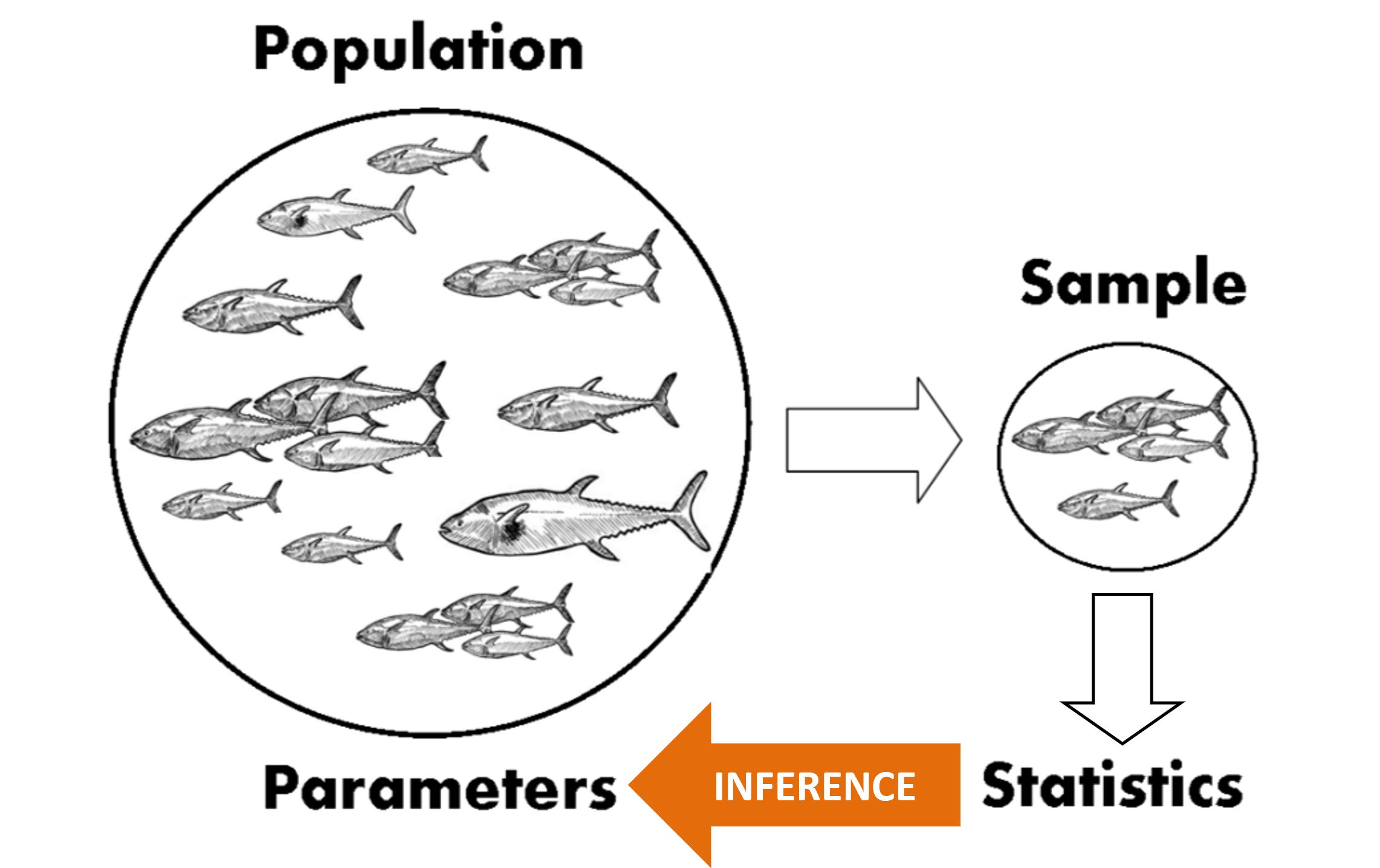
The term statistical inference means that we are using properties of a sample to make statements about the population from which the sample was drawn.
For example, say you wanted to know the mean length of the leaves on a tree (\(\mu\)). You wouldn’t want to (nor need to) measure every single leaf! You would take a random sample of leaves and measure their lengths (\(x_i\)), calculate the sample mean (\(\bar x\)), and use \(\bar x\) as an estimate of \(\mu\).
Statistical Inference for a Population Mean
Consider a population \(X\) with mean \(\mu\),
variance \(\text{Var}(X)=\sigma^2\), and
standard deviation \(\sigma\).
We can estimate \(\mu\) by:
taking a random sample of values \(\{x_1, x_2, ..., x_n\}\) from the population, \(X\), and
calculating the sample mean \(\bar x = \frac 1 n \sum_{i=1}^{n}x_i\).
Importantly:
The sample mean \(\bar x\) is a single draw from a random variable \(\bar X\). It will never be exactly equal to the population mean, \(\mu\), unless you measure every single leaf.
There is uncertainty in our estimate of \(\mu\). Each sample yields a different \(\bar x\). This is called sampling error.
Sampling Variation
Sampling Error
The variability of the sample means from sample to sample, \(\text{Var}(\bar X)\), depends on two things:
the variability of the population values, \(\text{Var}(x)\), and
the size of the sample, \(n\).
The variability of the sample estimate of a parameter is usually expressed as a standard error (SE), which is simply the theoretical standard deviation of \(\bar X\) from sample to sample.
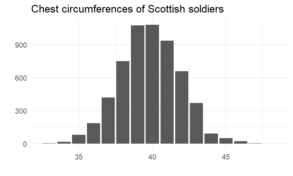
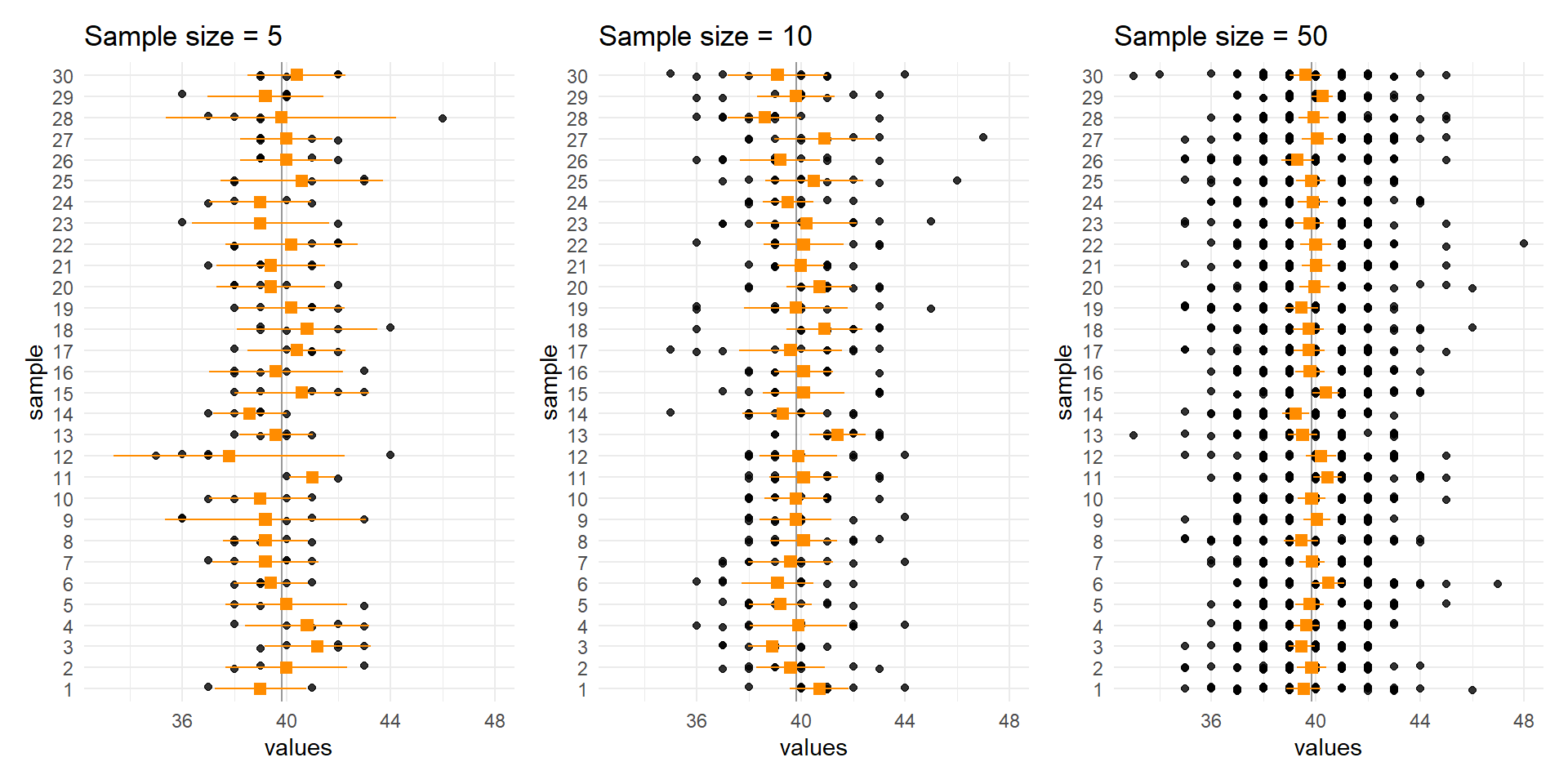
In 1846, a Belgian scholar Adolphe Quetelet published an analysis of the chest sizes of a full population of 5,738 Scottish soldiers.
The distribution of the measurements (in inches) in his database has a mean of \(\mu\) = 39.83 inches, a standard deviation of \(\sigma\) = 2.05 inches, and is well approximated by a normal distribution.
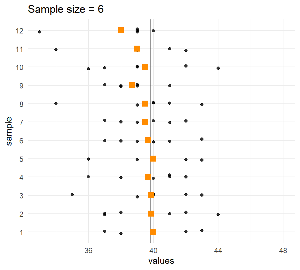
Every soldier was measured so we can treat this as the population, and \(\mu\) = 39.83 and \(\sigma\) = 2.05 as population parameters. Let’s take some samples of size \(n\) = 6 from this population.
# Convert to a long vector of valuesqd_long <-rep(qd$Chest, qd$Count)
Every soldier was measured so we can treat this as the population, and \(\mu\) = 39.83 and \(\sigma\) = 2.05 as population parameters. Let’s take some samples of size \(n\) = 6 from this population.
# Convert to a long vector of valuesqd_long <-rep(qd$Chest, qd$Count)
# Put ten samples in a tibbleq_samples <-tibble( sample =as_factor(1:10) ) |>mutate( values =map(sample, ~sample(qd_long, size =6)) ) |>unnest()head(q_samples, 15)
Every soldier was measured so we can treat this as the population, and \(\mu\) = 39.83 and \(\sigma\) = 2.05 as population parameters. Let’s take some samples of size \(n\) = 6 from this population.
# Convert to a long vector of valuesqd_long <-rep(qd$Chest, qd$Count)
# Put ten samples in a tibbleq_samples <-tibble( sample =as_factor(1:10) ) |>mutate( values =map(sample, ~sample(qd_long, size =6)) ) |>unnest()
# Calculate means of each samplesample_means <- q_samples |>group_by(sample) |>summarise(mean =mean(values))sample_means
The larger the \(n\), the less the sample means vary.
Standard error
If is distributed as a normal random variable with mean \(\mu\) and variance \(\sigma^2\),
\[X \sim \text{Normal}(\mu, \sigma)\]
then sample means of size \(n\) are distributed as
\[\bar X \sim \text{Normal}(\mu_\bar{X} = \mu, \sigma_\bar{X} = \sigma/\sqrt{n})\]\(\text{SE}(\bar{X}) = \sigma_\bar{X}= \sigma/\sqrt{n})\) is known as the standard error of the sample mean.
More generally, a standard error is the standard deviation of an estimated parameter over \(\infty\) theoretical samples.
According to the Central Limit Theorem (CLT), raw \(X\) values don’t have to be normally distributed for the sample means to be normally distributed (for any decent sample size)!
Quetelet’s chests: Standard error of means of samples
Question:
If Quetelet’s chest circumferences are distributed as \(X \sim \text{N}(\mu=39.83, \sigma=2.05)\), then how variable are the means of samples of size \(n\) = 6?
Answer:
\[
\begin{aligned}
SE(\bar{X}_{n=6})&=\sigma/\sqrt{n} \\
&=2.05/\sqrt{6} \\
&=0.8369
\end{aligned}
\] Sample means of size \(n\) = 6 would be distributed as
Quetelet’s chests: Distribution of means of samples
Confidence intervals
Another common way of expressing uncertainty when making statistical inferences is to present:
a point estimate (e.g., the sample mean) and
a confidence interval around that estimate.
A confidence interval gives an indication of the sampling error.
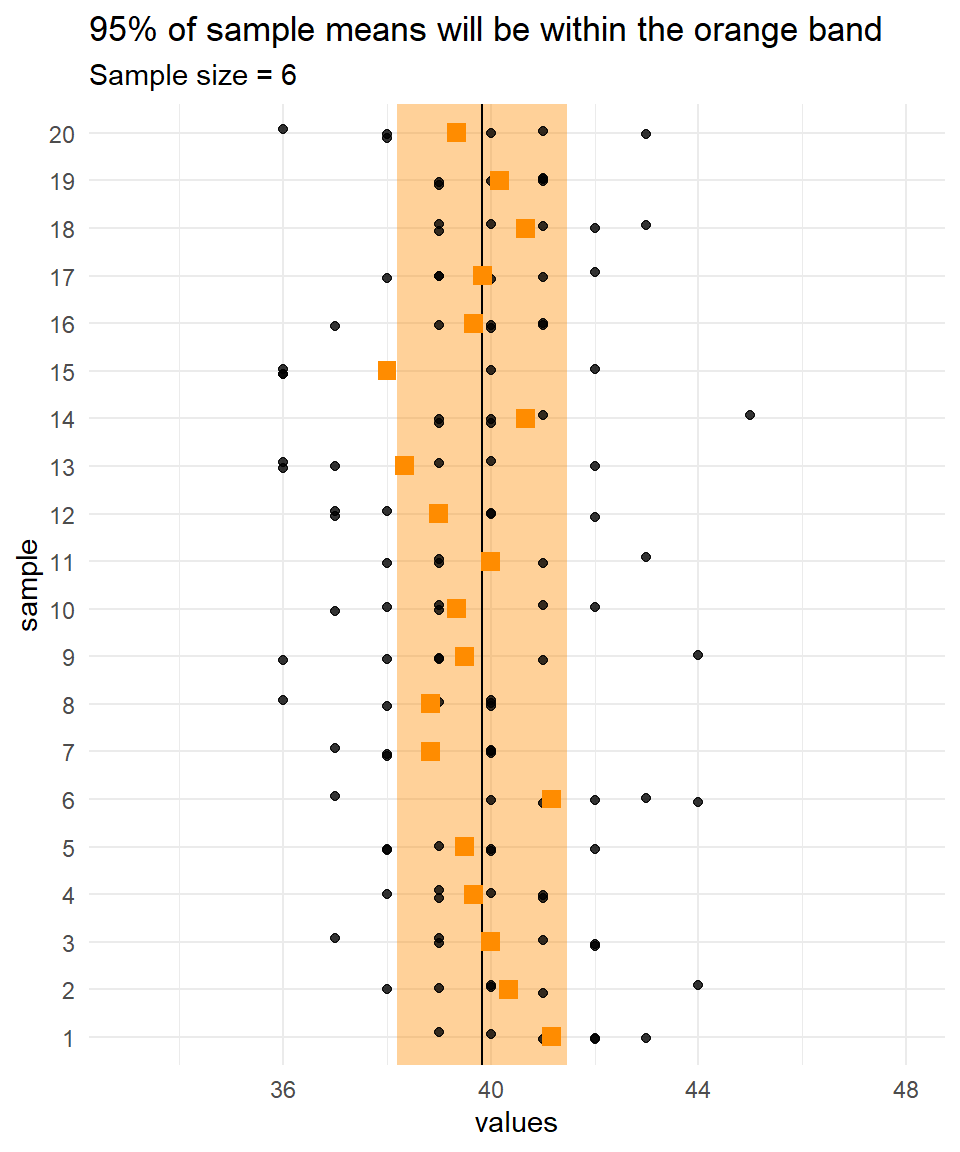
A 95% confidence interval is constructed so that intervals from 95% of samples will contain the true population parameter.
In reality the interval either contains the true value or not, so you must not interpret a confidence interval as “there’s a 95% probability that the interval contains the true parameter”.
We can say:
“95% of so-constructed intervals will contain the true value of the parameter” or
“with 95% confidence, the interval contains the true value of the parameter”.
Confidence intervals
Because we know the population parameters for the Quetelet dataset, we can calculate where 95% of sample means will lie for any particular sample size.
Recall that, for a normal distribution, 95% of values lie between \(\mu \pm 1.96\times\sigma\)
(i.e., \(\mu - 1.96\times\sigma\) and \(\mu + 1.96\times\sigma\)).
It follows that 95% of means of samples of size \(n\) will lie within \(\mu \pm 1.96 \times \sigma/\sqrt{n}\).
For example, for samples of size 6 from the Quetelet dataset, 95% of means will lie within \(39.83 \pm 1.96\times 2.05 / \sqrt 6\),
so \(\{ 37.02 , 42.64\}\).
Estimating the distribution of sample means from data
It’s all very well deriving the distribution of sample means when we know the population parameters (\(\mu\) and \(\sigma\)) but in most cases we only have our one sample.
We don’t know any of the population parameters. We have to estimate the population mean (usually denoted \(\hat\mu\) or \(\bar x\)) and estimate of the population standard deviation (usually denoted \(\hat\sigma\) or \(s\)) from the sample data.
This additional uncertainty complicates things a bit. In fact, we can’t even use the normal distribution any more!
The t distribution
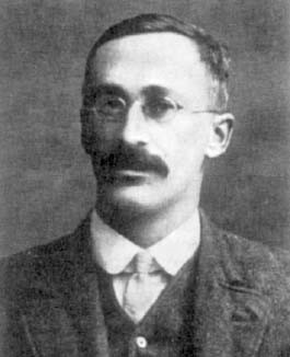
Introducing William Sealy Gosset, who described the t distribution after working with random numbers.
Gosset was a chemist and mathematician who worked for the Guinness brewery in Dublin.
Guinness forbade anyone from publishing under their own names so that competing breweries wouldn’t know what they were up to, so he published his discovery in 1908 under the penname “Student”. Student’s identity was only revealed when he died. It is therefore often called “Student’s t distribution”.
Willam Sealy Gosset 1876-1937
The t distribution
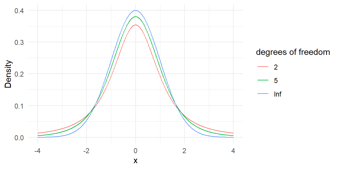
The t distribution is like the standard normal. It is bell-shaped and symmetric with mean = 0, but it has fatter tails (greater uncertainty) due to the fact that we do not know\(\sigma\); we have to estimate it.
The t distribution is not just a single distribution. It is really an entire series of distributions which is indexed by something called the “degrees of freedom” (or \(df\)).
As \(df \rightarrow \infty\), \(t \rightarrow Z\).
p <-expand_grid(df =c(2, 5, Inf),x =seq(-4, 4, by = .01) ) |>mutate(Density =dt(x = x, df = df),`degrees of freedom`=as_factor(df) ) |>ggplot() +aes(x = x, y = Density, group =`degrees of freedom`, colour =`degrees of freedom`) +geom_line()
The t distribution
For a sample of size \(n\), if
\(X\) is a normal random variable with mean \(\mu\),
\(\bar X\) is the sample mean, and
\(s\) is the sample standard deviation,
then the variable:
\[
T = \frac{\bar X - \mu} {s/\sqrt{n}}
\]
is distributed as a \(t\) distribution with \((n – 1)\) degrees of freedom.
Confidence intervals and the t distribution
The process of using sample data to try and make useful statements about an unknown parameter, \(\theta\), is called statistical inference.
A confidence interval for the true value of a parameter is often obtained by:
\[
\hat \theta \pm t \times \text{SE}(\hat \theta)
\] where \(\hat \theta\) is the sample estimate of \(\theta\) and \(t\) is a quantile from the \(t\) distribution with the appropriate degrees of freedom.
For example, to get the \(t\) score for a 95% confidence interval with 9 degrees of freedom:
qt(p =0.975, df =9)
[1] 2.262157
The piece that is being added and subtracted, \(t \times \text{SE}(\hat \theta)\), is often called the margin of error.
Confidence intervals for a sample mean
We can calculate a 95% confidence interval for a sample mean with the following information:
sample mean \(\bar x\),
sample standard deviation \(s\),
the sample size \(n\), and
the 0.025th quantile of the \(t\) distribution with degrees of freedom \(df=n-1\).
    One Sample t-test

data:  dq1
t = 46.6, df = 5, p-value = 8.595e-08
alternative hypothesis: true mean is not equal to 0
95 percent confidence interval:
 36.69118 40.97548
sample estimates:
mean of x
 38.83333
Confidence intervals for sample means
t as a test statistic
This method can be used when the estimator \(\hat\theta\) is approximately normally distributed and
This paves the way for hypothesis testing for specific values of \(\theta\). Many of the methods you will learn in this course are based on this general rule.
Testing hypotheses
Testing hypotheses underpins a lot of scientific work.
A hypothesis is a proposition, a specific idea about the state of the world that can be tested with data.
For logical reasons, instead of measuring evidence for a hypothesis of interest, scientists will often:
specify a null hypotheses, which must be true if our hypothesis of interest is false, and
measure the evidence against the null hypothesis, usually in the form of a p-value.
Example: growth of alfalfa
Say a farmer has 9 paddocks of alfalfa. He’s hired a new manager, and wants to know if, on average, this year’s crop is different to last year’s. He measures the yield for each paddock in year 1 and year 2, and calculates the difference.
The mean difference is 0.067. On average, yields were 0.067 greater than last year.
Is that convincing different from zero?
How likely is such a difference to have arisen just by chance, and really, if we had a million paddocks, there would be no difference?
What is the probability of seeing a difference of 0.067 or more in our dataset if the true mean were zero?
These questions can be addressed with a \(p\)-value from a hypothesis test.
Example: growth of alfalfa
The hypothesis of interest (called the “alternative” hypothesis) is:
\(\ \ \ \ \ H_A: \mu \ne 0\), that is, the mean difference in yield \(\mu\) between the two years is not zero.
The null hypothesis (the case if the alternative hypothesis is wrong) is:
\(\ \ \ \ \ H_0: \mu = 0\), that is, the mean difference is zero.
We can test the null hypothesis using a t statistic \(t_0 = \frac{\bar x - \mu_0} {\text{SE}(\bar x)}\), where \(\ \ \ \ \ \mu_0 = 0\) is the hypothesised value of the mean and \(\ \ \ \ \ \text{SE}(\bar x) = s/\sqrt{n}\) is the (estimated) standard error of the sample mean.
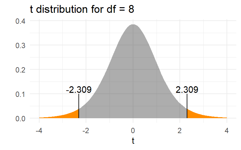
( t0 <- (xbar -0) / ( s /sqrt(9) ) )
[1] 2.309401
The p-value is \(\text{Pr}(|t_{df=8}| > t_0)\)
2*pt(t0, df =8, lower = F)
[1] 0.04973556
Example: growth of alfalfa
The hypothesis of interest (called the “alternative” hypothesis) is:
\(\ \ \ \ \ H_A: \mu \ne 0\), that is, the mean difference in yield \(\mu\) between the two years is not zero.
The null hypothesis (the case if the alternative hypothesis is wrong) is:
\(\ \ \ \ \ H_0: \mu = 0\), that is, the mean difference is zero.
This can be done more easily:
t.test(diff)
    One Sample t-test

data:  diff
t = 2.3094, df = 8, p-value = 0.04974
alternative hypothesis: true mean is not equal to 0
95 percent confidence interval:
 9.806126e-05 1.332353e-01
sample estimates:
 mean of x
0.06666667
Example: growth of alfalfa
The \(p\)-value of 0.05 means that, if the null hypothesis were true, only 5% of sample means would be as or more extreme than the observed value of 0.067. It is the area in orange in the graph below.
We can therefore reject the null hypothesis at the conventional 5% level, and conclude that, on average, yields were indeed higher this year.
This is an example of a paired t test. They two samples (year 1 and year 2) are not independent of one another because we have the same paddocks in both years. So, we take the differences, treat them like a single sample, and do a one-sample t test for the mean difference being zero.
In reality, the null hypothesis is either true or false.
The outcome of a test is either we reject the null hypothesis, or we fail to reject the null hypothesis (note, we never “confirm” or “accept” the null hypothesis – absence of evidence is not evidence of absence!).
This gives us four possibilities:
\(H_0\) is true
\(H_0\) is false
Reject \(H_0\)
Type I error
Correct result
Do not reject \(H_0\)
Correct result
Type II error
With probabilities usually represented by:
\(H_0\) is true
\(H_0\) is false
Reject \(H_0\)
\(\alpha\)
\(1-\beta\) = “power”
Do not reject \(H_0\)
\(1 - \alpha\)
\(\beta\)
Truth and outcomes
The probability of making a Type I error, rejecting \(H_0\) when \(H_0\) is true, is set by the experimenter a priori (beforehand) as the significance level, \(\alpha\).
Say we set \(\alpha\) at the conventional 0.05. We know that, if \(H_0\) is true, we have a 5% chance of rejecting \(H_0\) (the Type I error rate is 0.05) and a 95% chance of not rejecting \(H_0\).
The probability of retaining (not rejecting) \(H_0\) when \(H_0\) is false is usually represented by \(\beta\) (“beta”).
We usually do not know \(\beta\) because it depends on \(\sigma\), \(n\) and also the effect size under the alternative hypothesis. These must be asserted to calculate \(\beta\) and power, \(1-\beta\).
Calculating power
The power of a hypothesis test is the probability of rejecting the null hypothesis if it is indeed false. Basically, “if we’re right, what is the probability that we’ll be able to show it?”
The power of the \(t\) test can be evaluated using R if you assert the effect size \(\delta\):
     Two-sample t test power calculation

              n = 10
          delta = 1
             sd = 1
      sig.level = 0.05
          power = 0.5619846
    alternative = two.sided

NOTE: n is number in *each* group
     Two-sample t test power calculation

              n = 50
          delta = 1
             sd = 1
      sig.level = 0.05
          power = 0.9986074
    alternative = two.sided

NOTE: n is number in *each* group
The bigger the sample size, the bigger more power we have to detect an effect.
Often, experimenters might aim to have a power of 80% or more, so they will most likely reject the null if it is false.
Sampling distributions
The term sampling distribution means the distribution of the computed statistic such as the sample mean when sampling is repeated many times.
For a normal population,
Student’s \(t\) distribution is the sampling distribution of the mean (after rescaling).
\(\chi^2\) distribution is the sampling distribution of the sample variance \(S^2\).
\(F\) distribution is ratio of two \(\chi^2\) distributions.
It becomes the sampling distribution of the ratio of two sample variances \(S_1^2/S_2^2\) from two normal populations (after scaling).
\(t\) distribution is symmetric but \(\chi^2\) and \(F\) distributions are right skewed. - For large samples, they become normal - For \(n>30\), the skew will diminish
For the three sampling distributions, the sample size \(n\) becomes the proxy parameter, called the degrees of freedom (df).
The two-sample t-test is a common statistical test. You have two populations, \(X_1\) and \(X_2\), with means \(\mu_1\) and \(\mu_2\) and variances \(\sigma^2_1\) and \(\sigma^2_2\), respectively.
We wish to test whether the two population means are equal.
Null hypothesis: \(H_0:\mu=\mu_1=\mu_2\)
Two-sided alternative hypothesis: \(H_1:\mu_1 \neq \mu_2\)
The basic t-test assumes equal variances; that is, \(\sigma^2_1 = \sigma^2_2\).
If we make this assumption and it is false, the test may give the wrong conclusion!
Two sample t-test with equal variances
Under the assumption of equal variances \(\sigma^2_1 = \sigma^2_2\), we can perform a pooled-sample t-test.
We calculate the estimated pooled variance as:
\[s_{p}^{2} = w_{1} s_{1}^{2} +w_{2} s_{2}^{2}\]
where the weights are \(w_{1} =\frac{n_{1}-1}{n_{1} +n_{2}-2}\) and \(w_{2} =\frac{n_{2}-1}{n_{1} +n_{2}-2}\),
and \(n_1\) and \(n_2\) are the sample sizes for samples 1 and 2, respectively.
For the pooled case, the \(df\) for the \(t\)-test is simply
\[df = n_{1}+n_{2}-2\]
Two sample t-test with unequal variances
This is often called the “Welch test”.
We do not need to calculated the pooled variance \(s^2_p\);
we simply use \(s^2_1\) and \(s^2_2\) as they are.
For the unpooled case, the \(df\) for the test is smaller: \[df=\frac{\left(\frac{s_{1}^{2}}{n_{1}} +\frac{s_{2}^{2} }{n_{2}} \right)^{2} }{\frac{1}{n_{1} -1} \left(\frac{s_{1}^{2}}{n_{1}}\right)^{2} +\frac{1}{n_{2} -1} \left(\frac{s_{2}^{2}}{n_{2} } \right)^{2}}\] The \(df\) doesn’t have to be an integer in this case.
Validity of equal variance assumption
We can test the null hypothesis that the variances are equal using either a Bartlett’s test or Levene’s test. Levene’s is generally favourable over Bartlett’s.
tv =read_csv("https://www.massey.ac.nz/~anhsmith/data/tv.csv")car::leveneTest(TELETIME~factor(SEX), data=tv)
Levene's Test for Homogeneity of Variance (center = median)
      Df F value  Pr(>F)
group  1  3.1789 0.08149 .
      44
---
Signif. codes:  0 '***' 0.001 '**' 0.01 '*' 0.05 '.' 0.1 ' ' 1
Highish p-value means there’s no strong evidence against the null hypothesis that the variances are equal. Therefore, we might feel happy to assume equal variances and use a pooled variance estimate.
    Two Sample t-test

data:  TELETIME by factor(SEX)
t = -0.7249, df = 44, p-value = 0.4723
alternative hypothesis: true difference in means between group 1 and group 2 is not equal to 0
95 percent confidence interval:
 -461.3476  217.2606
sample estimates:
mean in group 1 mean in group 2
       1668.261        1790.304
t-test not assuming equal variances (Welch test):
t.test(TELETIME ~factor(SEX), data=tv)
    Welch Two Sample t-test

data:  TELETIME by factor(SEX)
t = -0.7249, df = 40.653, p-value = 0.4727
alternative hypothesis: true difference in means between group 1 and group 2 is not equal to 0
95 percent confidence interval:
 -462.1384  218.0514
sample estimates:
mean in group 1 mean in group 2
       1668.261        1790.304
For more on non-parametric tests, see Study Guide.
Test of proportions
Testing the null hypothesis that a proportion \(p=0.5\)
Alternative hypothesis: \(p \ne 0.5\)
Say a survey of 1000 beached whales had 450 females.
Is the population 50:50?
prop.test(450, 1000)
    1-sample proportions test with continuity correction

data:  450 out of 1000, null probability 0.5
X-squared = 9.801, df = 1, p-value = 0.001744
alternative hypothesis: true p is not equal to 0.5
95 percent confidence interval:
 0.4189204 0.4814685
sample estimates:
   p
0.45
An exact version of the test
binom.test(c(450, 550))
    Exact binomial test

data:  c(450, 550)
number of successes = 450, number of trials = 1000, p-value = 0.001731
alternative hypothesis: true probability of success is not equal to 0.5
95 percent confidence interval:
 0.4188517 0.4814435
sample estimates:
probability of success
                  0.45
To test for a proportion other than 0.5
binom.test(c(450, 550), p =3/4)
    Exact binomial test

data:  c(450, 550)
number of successes = 450, number of trials = 1000, p-value < 2.2e-16
alternative hypothesis: true probability of success is not equal to 0.75
95 percent confidence interval:
 0.4188517 0.4814435
sample estimates:
probability of success
                  0.45
Comparing several proportions
Data on smokers in four group of patients
(from Fleiss, 1981, Statistical methods for rates and proportions).
    4-sample test for equality of proportions without continuity correction

data:  smokers out of patients
X-squared = 12.6, df = 3, p-value = 0.005585
alternative hypothesis: two.sided
sample estimates:
   prop 1    prop 2    prop 3    prop 4
0.9651163 0.9677419 0.9485294 0.8536585
More on chi-squared tests next week.
Tests for normality
Testing the hypothesis that sample data came from a normally distributed population. \(H_0: X \sim N(\mu, \sigma)\).
Kolmogorov-Smirnov test (based on the biggest difference between the empirical and theoretical cumulative distributions)
Shapiro-Wilk test (based on variance of the difference)
Example: a sample of \(n\) = 50 from N(100,1).
set.seed(123)shapiro.test(rnorm(50, mean=100))
    Shapiro-Wilk normality test

data:  rnorm(50, mean = 100)
W = 0.98928, p-value = 0.9279
set.seed(123)ks.test(rnorm(50), "pnorm")
    Exact one-sample Kolmogorov-Smirnov test

data:  rnorm(50)
D = 0.073034, p-value = 0.9347
alternative hypothesis: two-sided
The large p-values mean that there’s no evidence of non-normality.
Like all tests, they can give the wrong answer. Try with set.seed(1234).
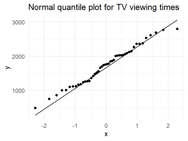
Can also use plots to assess normality
tv =read_csv("https://www.massey.ac.nz/~anhsmith/data/tv.csv")ggplot(tv, aes(sample = TELETIME)) +stat_qq() +stat_qq_line() +labs(title ="Normal quantile plot for TV viewing times")
Transformations
It can be useful to transform skewed data to make the distribution more like a ‘normal’ if that is required for a particular analysis.
A linear transformation \(Y^*= a+bY\) only changes the scale or centre, not the shape of the distribution.
Transformations can help to improve symmetry, normality, and stabilise the variance.
Example
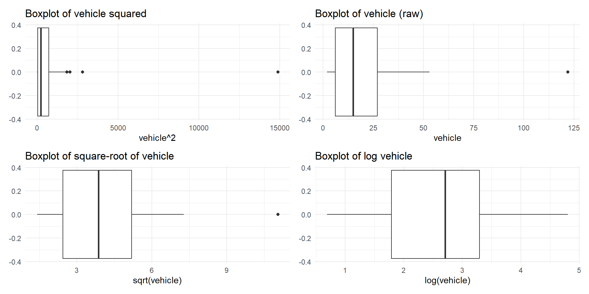
Right skewed distribution is made roughly symmetric using a log transformation for no. of vehicles variable (rangitikei.* dataset)
A Ladder of Powers for Transforming Data
Right skewed data needs a shrinking transformation
Left skewed data needs a stretching transformation
The strength or power of the transformation depends on the degree of skew.
POWER
Formula
Name
Result
3
\(x^3\)
cube
stretches large values
2
\(x^2\)
square
stretches large values
1
\(x\)
raw
No change
1/2
\(\sqrt{x}\)
square root
squashes large values
0
\(\log{x}\)
logarithm
squashes large values
-1/2
\(\frac{-1}{\sqrt{x}}\)
reciprocal root
squashes large values
-1
\(\frac{-1}{x}\)
reciprocal
squashes large values
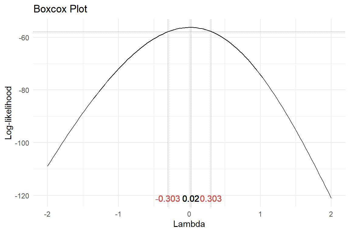
Box-Cox transformation
This is a normalising transformation based on the Box-Cox power parameter, \(\lambda\).
R gives a point estimate of the Box-Cox power & a confidence interval.
Usually, we are concerned about whether the residuals from a model are normally distributed – put the model in the lm statement.
Sometimes, no “good” value of \(\lambda\) can be found.
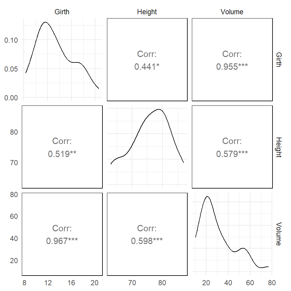
Figure 1: Comparison of Pearsonian and Spearman’s rank correlations
Wilcoxon signed rank test
A non-parametric alternative to the one-sample t-test
\(H_0: \eta=\eta_0\) where \(\eta\) (Greek letter ‘eta’) is the population median
Based on based on ranking \((|Y-\eta_0|)\), where the ranks for data with \(Y<\eta_0\) are compared to the ranks for data with \(Y>\eta_0\)
wilcox.test(tv$TELETIME, mu=1680, conf.int=T)
    Wilcoxon signed rank exact test

data:  tv$TELETIME
V = 588, p-value = 0.6108
alternative hypothesis: true location is not equal to 1680
95 percent confidence interval:
 1557.5 1906.5
sample estimates:
(pseudo)median
          1728
t.test(tv$TELETIME, mu=1680)
    One Sample t-test

data:  tv$TELETIME
t = 0.58856, df = 45, p-value = 0.5591
alternative hypothesis: true mean is not equal to 1680
95 percent confidence interval:
 1560.633 1897.932
sample estimates:
mean of x
 1729.283
Mann-Whitney test
For two group comparison, pool the two group responses and then rank the pooled data
Ranks for the first group are compared to the ranks for the second group
The null hypothesis is that the two group medians are the same: \(H_0: \eta_1=\eta_2\).
    Wilcoxon rank sum test with continuity correction

data:  rangitikei$people by rangitikei$time
W = 30, p-value = 0.007711
alternative hypothesis: true location shift is not equal to 0
95 percent confidence interval:
 -88.99996 -10.00005
sample estimates:
difference in location
             -36.46835
t.test(rangitikei$people~rangitikei$time)
    Welch Two Sample t-test

data:  rangitikei$people by rangitikei$time
t = -3.1677, df = 30.523, p-value = 0.003478
alternative hypothesis: true difference in means between group 1 and group 2 is not equal to 0
95 percent confidence interval:
 -102.28710  -22.13049
sample estimates:
mean in group 1 mean in group 2
       22.71429        84.92308
Another form of test
kruskal.test(rangitikei$people~rangitikei$time)
    Kruskal-Wallis rank sum test

data:  rangitikei$people by rangitikei$time
Kruskal-Wallis chi-squared = 7.2171, df = 1, p-value = 0.007221
wilcox.test(rangitikei$people~rangitikei$time)
    Wilcoxon rank sum test with continuity correction

data:  rangitikei$people by rangitikei$time
W = 30, p-value = 0.007711
alternative hypothesis: true location shift is not equal to 0
Permutation tests
A permutation (or randomisation) test has the following steps:
Randomly permute the observed data many times, thereby destroying any real relationship,
Recalculate the test statistic \(T\) for each random permutation
Compare the observed value of \(T\) (from the actual data) with the values of \(T\) under permutation.
[1] "Settings: unique SS : numeric variables centered"
Call:
lmp(formula = TELETIME ~ SEX, data = tv)

Residuals:
      Min        1Q    Median        3Q       Max
-1178.261  -510.793    -7.283   402.989  1130.739

Coefficients:
    Estimate Iter Pr(Prob)
SEX      122   51     0.98

Residual standard error: 570.9 on 44 degrees of freedom
Multiple R-Squared: 0.0118, Adjusted R-squared: -0.01066
F-statistic: 0.5255 on 1 and 44 DF,  p-value: 0.4723
Read the study guide example for bootstrap tests (not examined)
Summary
Basic methods of inference include:
estimating a population parameter (e.g. mean) using a sample of values,
estimating standard deviation of a sample estimate using the standard error,
constructing confidence intervals for an estimate, and
testing hypotheses about particular values of the population parameter.
Inference is relatively easy for normally distributed populations.
Student’s t-tests include:
one-sample t-test, including paired-sample t-test for a difference of zero
two-sample t-test assuming equal variances (estimating pooled variance)
two-sample t-test not assuming equal variances (Welch test)
The t-test is generally robust for non-normal populations (especially for large samples).
Power transformations, such as square-root, log, or Box-Cox aim to reduce skewness.
Non-parametric tests can be used for non-normal data, but they are usually less powerful than parametric tests.